1. Introduction to Running K2Taxonomer (Bulk Expression Data)
Eric R. Reed
Boston University School of Medicine, Section of Computational Biomedicine, 72 E Concord St, Boston, MA 02118reeder@bu.edu
October 21, 2020
Source:vignettes/RunningK2Taxonomer.Rmd
RunningK2Taxonomer.RmdIntroduction
This vignette describes the general workflow for running K2Taxonomer on gene expression data (Reed and Monti 2020). While this vignette describes an analysis of bulk gene expression data, many of these steps are shared with that of single-cell expression analyses. A vignette for running K2Taxonomer on single-cell expression data can be found here.
Requirements
Read in sample ExpressionSet object
The main input of K2Taxonomer is an ExpressionSet object with approximately normally distributed expression values. Here we read in an example data set. See ?sample.ExpressionSet for more information about these data.
data(sample.ExpressionSet)K2Taxonomer basic run
Initialize K2 object
The K2preproc() initializes the K2 object and runs pre-processing steps. Here, you can specify all arguments used throughout the analysis. Otherwise, you can specify these arguments within the specific functions for which they are implemented. See help pages for more information.
Here we will start by using the defaults.
## Run pre-processing
K2res <- K2preproc(sample.ExpressionSet)
Note: This data set is microarray expression data. If using normalized and log-transformed count data then it’s generally recommended that you set logCounts=TRUE . This will more appropriately perform differential gene expression analyses with the limma R package (Ritchie et al. 2015).
## NOT RUN
K2res <- K2preproc(sample.ExpressionSet,
                    logCounts=TRUE)
K2 object structre
K2Taxonomer functions create and manipulate S4, K2 objects, defined within the package. K2 objects have 5 slots.
-
eSet: “ExpressionSet”: Original expression data, extracted by
K2eSet(). -
meta: “list”: Named list of parameters for running analysis, extracted by
K2data(). -
dataMatrix: “matrix”: Matrix of processed expression data for running K2Taxonomer algorithm, extracted by
K2results. -
info: “data.frame”: Data frame of entered observation-level information, extracted by
K2info(). -
results: “list”: Named list of the results of running the K2Taxonomer algorithm, including differential analysis and enrichment results, extracted by
K2results() -
genesets: “list”: Named list of gene sets to run for enrichment analysis, extracted by
K2genesets. -
gene2Pathway: “character”: Named vector of gene set names in which each gene appears, extracted by
K2gene2Pathway. -
geneURL: “character”: Named vector of URLs to link to each gene in the dashboard, extracted by
K2geneURL(). -
genesetURL: “character”: Named vector of URLs to link to each gene set in the dashboard, extracted by
K2genesetURL().
K2preproc() will fill in three of these slots:, eSet, meta, and dataMatrix.
## Extract ExpressionSet
K2eSet(K2res)
#> ExpressionSet (storageMode: lockedEnvironment)
#> assayData: 500 features, 26 samples
#>   element names: exprs, se.exprs
#> protocolData: none
#> phenoData
#>   sampleNames: A B ... Z (26 total)
#>   varLabels: sex type score
#>   varMetadata: labelDescription
#> featureData: none
#> experimentData: use 'experimentData(object)'
#> Annotation: hgu95av2

## Extract dataMatrix
dim(K2data(K2res))
#> [1] 500  26
meta will be populated by default a set of parameters entered into K2preproc(). Note that for each step, new parameters may be entered, specific to that function.
## Extract meta data
names(K2meta(K2res))
#>  [1] "cohorts"          "vehicle"          "covariates"       "block"
#>  [5] "logCounts"        "infoClass"        "use"              "nFeats"
#>  [9] "featMetric"       "recalcDataMatrix" "nBoots"           "clustFunc"
#> [13] "clustCors"        "clustList"        "linkage"          "qthresh"
#> [17] "cthresh"          "ntotal"           "ssGSEAalg"        "ssGSEAcores"
#> [21] "oneoff"           "stabThresh"
Running K2Taxonomer algorithm
The K2Taxonomer is run by K2tax(). At each recursion of the algorithm, the observations in dataMatrix are partitioned into two sub-groups based on a compilation of repeated K=2 clustering on bootstrapped sampling of features. For each partition in the recursion, a stability metric is used to estimate robustness, which takes on values between 0 and 1, where values close to 1 represent the instance in which the same clustering occured in every or nearly every perturbation of a large set of observations. As the number of observations decreasing down the taxonomy the largest possible stability estimate decreases, such that the largest possible stability estimate of triplets and duplets, is 0.67 and 0.50, respectively.
The parameter, stabThresh, controls the minimum value of the stability metric to continue partitioning the observations. By default, stabThresh is set to 0, which will run the algorithm until until all observations fall into singlets. If we set stabThresh=0.5 the algorithm can not separate duplets, as well as larger sets that demonstrate poor stability when a partition is attempted. This can also be set during initialization with K2preproc().
Choosing an appropriate threshold is dependent on the size of the original data set. For large data sets, choosing small values will greatly increase runtime, and values between 0.8 and 0.7, are generally recommended.
## Run K2Taxonomer aglorithm
K2res <- K2tax(K2res,
            stabThresh=0.5)
K2Taxonomer results structure
The results slot of the K2 object is a named list of the results of running the K2Taxonomer algorithm. Each item in the list contains the IDs of the two sets of observations denoted by the partitions, as well as additional annotation for that partition, including the stability estimates.
Each item is assigned a letter ID. If there are more than 26 items, than an additional letter is tacked on, such that the 27th item is named, AA, and the 28th item is named BB.
Partition results
## Get observations defined in each partition
K2results(K2res)$A$obs
#> [[1]]
#>  [1] "A" "C" "D" "F" "G" "J" "M" "O" "Q" "R" "S" "U" "V" "W" "X"
#>
#> [[2]]
#>  [1] "B" "E" "H" "I" "K" "L" "N" "P" "T" "Y" "Z"
Stability metrics
Stability metrics measure the extant to which pairs of observations in the data setpartitioned together for a given partition of the data.
## Get bootstrap probability of this partition
K2results(K2res)$A$bootP
#> [1] 0.05

## Node stability (Value between 0 and 1. 1 indicating high stability)
K2results(K2res)$A$stability$node
#> [1] 0.6974732

## Stability of each subseqent subgroup.
K2results(K2res)$A$stability$clusters
#> [1] 0.6516701 0.7071291

## Distance matrix indicating pairwise cosine similarity of each observation
partitionAstability <- as.matrix(K2results(K2res)$A$stability$samples)

## Show heatmap
hcols <- c("grey", "black")[colnames(partitionAstability) %in%
    K2results(K2res)$A$obs[[1]] + 1]

heatmap(partitionAstability,
        distfun=function(x) as.dist(1-x),
        hclustfun=function(x) hclust(x, method="mcquitty"),
        col=hcl.colors(12, "Blue-Red"),
        scale="none",
        cexRow=0.7,
        cexCol=0.7,
        symm=TRUE,
        ColSideColors=hcols,
        RowSideColors=hcols,
        keep.dendro=FALSE)
Generate dendrogram from K2Taxonomer results
After running the K2Taxonomer algorithm, a dendrogram object can be built using K2dendro().
## Get dendrogram from K2Taxonomer
dendro <- K2dendro(K2res)

## Get dendrogram data
ggdendrogram(dendro)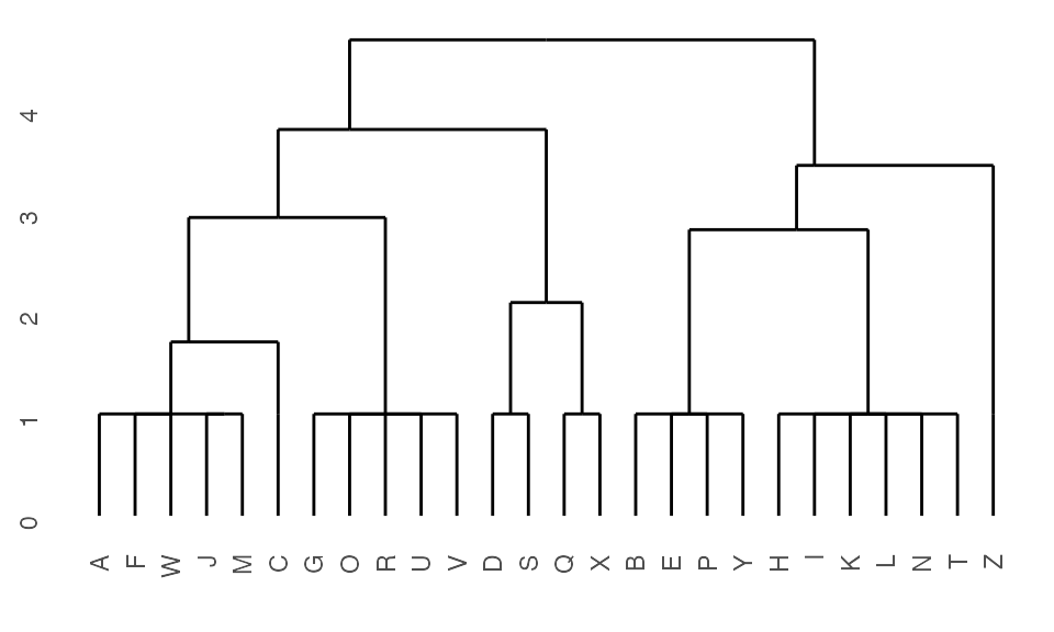
Annotating K2Taxonomer results
A principal motivation behind K2Taxonomer is that insight can be garnered and tracjed for various levels in a hierarchical sub-grouping of obervations, such that analytical characterization of different sub-groups throughout the taxonomy serve to both validate and inform about specific sub-groups.
To this end, K2Taxonomer runs additional analyses to annotate each partition. These analyses include: differential expression analysis using the limma package and gene set enrichment testing for both hyperenrichment and differntial analysis of singe-sample enrichment scores estimated using the GSVA package (Ritchie et al. 2015)(Hanzelmann, Castelo, and Guinney 2013).
Differential gene expression analysis
Differential analysis in K2Taxonomer is performed using limma. Differential analysis is performed for each partition of the data, comparing the gene expression between each pair of subgroups across all partitions.
## Run DGE
K2res <- runDGEmods(K2res)

## Get differential results for one partition
head(K2results(K2res)$A$dge)
#>                        gene       coef       mean        t         pval
#> 1                  31492_at  282.13664  307.98895 6.955755 2.796513e-07
#> 2                  31461_at   27.57876   41.53356 5.633815 7.423551e-06
#> 3 AFFX-HUMGAPDH/M33197_5_at 1709.65597 2262.19365 5.398349 1.354315e-05
#> 4                  31321_at   36.15622  141.04954 5.358643 1.499377e-05
#> 5                  31385_at 1202.02188 3490.16038 5.169070 2.440299e-05
#> 6                31675_s_at   33.12332   30.28507 5.020459 3.579310e-05
#>           fdr         B edge
#> 1 0.000740363 -2.520401    2
#> 2 0.004708729 -2.879747    1
#> 3 0.005417262 -2.954549    2
#> 4 0.005452282 -2.967498    1
#> 5 0.006972284 -3.030659    2
#> 6 0.007954022 -3.081715    2

## Concatenate all results and generate table
DGEtable <- getDGETable(K2res)
head(DGEtable)
#>             gene      coef       mean         t         pval         fdr
#> 1       31492_at 282.13664  307.98895  6.955755 2.796513e-07 0.000740363
#> 2       31397_at  93.10100   39.35873 11.829624 3.701815e-07 0.000740363
#> 3       31589_at 195.18564   97.21551 10.249751 1.385089e-06 0.001846785
#> 4     31596_f_at 900.65933 1468.05440 10.679512 2.232714e-06 0.002232714
#> 5       31461_at  27.57876   41.53356  5.633815 7.423551e-06 0.004708729
#> 6 AFFX-PheX-3_at  87.55050   25.75616  8.497926 7.429352e-06 0.004708729
#>           B edge node direction
#> 1 -2.520401    2    A        up
#> 2 -4.318449    2    C        up
#> 3 -4.325216    2    C        up
#> 4 -3.953010    1    F        up
#> 5 -2.879747    1    A        up
#> 6 -4.336824    1    C        up
See ?getDGETable for a description of the columns in this data frame.
Interpretting differential analysis results
In this example, we are running K2Taxonomer without information specifying a set of observations to treat as a control group, for which to make comparisons in regards to the directionality of differential expression. In the absence of this designation, K2Taxonomer assigns genes to the partition-specific subgroup with the larger mean. Accordingly, the of coeficient (the “coef” in the output of getDGETable()) is always positive, indicating the difference of mean of the gene expression of the assigned subgroup from the other subgroup. Moreover, the “direction” of this gene will always be assigned to up.
Following the full description of this analysis, we describe methods for running K2Taxonomer, specifying a cohort variable in the data set. When including this variable, the user may assign one of the levels of this variable as the control group. With the inclusion of this designation, K2Taxonomer will assign directionality to the differences in gene expression.
Gene set hyperenrichment
K2Taxonomer performed both hyperenrichment and differential single-sample enrichment tests based on an input of gene sets using the genesets argument, which can be specified in runGSEmods(), as demonstrated here, or during initialization with K2preproc(). Here, the gene sets are made up.
Gene set hyperenrichment is performed on the top genes for each subgroup, as defined by differential analysis with the runGSEmods(). The arguments qthresh and cthresh specify thresholds for defining top genes, based on FDR Q-value and log fold-change, respectively. Here, qthresh=0.1, such that genes with FDR Q-value < 0.1 will be assigned as the top genes for a given partition.
## Create dummy set of gene sets
genes <- unique(DGEtable$gene)
genesetsMadeUp <- list(
    GS1=genes[1:50],
    GS2=genes[51:100],
    GS3=genes[101:150])

## Run gene set hyperenrichment
K2res <- runGSEmods(K2res,
                genesets=genesetsMadeUp,
                qthresh=0.1)
Single-sample gene set enrichment
Single-sample enrichment is performed in two steps. First, the GSVA package is used to generate observation-level enrichment scores, followed by differential analysis using the limma package. This is performed by the functions runGSVAmods() and runDSSEmods(), respectively. Here, we can specify which enrichment algorithm to use when running the GSVA functionality and the number of CPU cores to use with the ssGSEAalg and ssGSEAcores arguments, respectively. These can also be set in the K2preproc() function. Note, that the arguments shown are the defaults.
## Create expression matrix with ssGSEA(GSVA) estimates
K2res <- runGSVAmods(K2res,
                    ssGSEAalg="gsva",
                    ssGSEAcores=1,
                    verbose=FALSE)

## Extract ernichment score Expression Set object
K2gSet(K2res)
#> ExpressionSet (storageMode: lockedEnvironment)
#> assayData: 3 features, 26 samples
#>   element names: exprs
#> protocolData: none
#> phenoData
#>   sampleNames: A B ... Z (26 total)
#>   varLabels: sex type score
#>   varMetadata: labelDescription
#> featureData: none
#> experimentData: use 'experimentData(object)'
#> Annotation:
Differential single-sample enrichment analysis
## Run differential analysis on enrichment score Expression Set
K2res <- runDSSEmods(K2res)

## Extract table of all hyper and sample-level enrichment tests
K2enrRes <- getEnrichmentTable(K2res)
head(K2enrRes)
#>   category node edge direction   pval_hyper    fdr_hyper nhits ndrawn ncats
#> 1      GS2    A    1        up 6.037924e-48 2.354790e-46    23     55    50
#> 2      GS1    A    2        up 6.857536e-43 1.337219e-41    18     26    50
#> 3      GS3    A    1        up 5.302699e-40 6.893509e-39    20     55    50
#> 4      GS1    C    2        up 1.291858e-29 1.259561e-28    14     31    50
#> 5      GS2    C    2        up 1.944106e-24 1.516403e-23    12     31    50
#> 6      GS1    A    1        up 5.794277e-21 3.766280e-20    12     55    50
#>    ntot   pval_limma    fdr_limma      coef         mean        t         B
#> 1 20000 8.223428e-05 9.868114e-04 0.2956151  0.012747508 4.481631  1.218911
#> 2 20000 1.672127e-03 1.003276e-02 0.3006322  0.003870370 3.418727 -1.660982
#> 3 20000 1.534239e-06 3.682173e-05 0.3393635  0.002788223 5.826365  5.088093
#> 4 20000 7.459682e-02 2.237905e-01 0.3140979  0.177312002 1.896258 -4.181043
#> 5 20000 2.868128e-02 1.147251e-01 0.3403289 -0.157799671 2.384535 -3.424011
#> 6 20000           NA           NA        NA           NA       NA        NA
#>                                                                                                                                                                                                                                                                  hits
#> 1 31428_at,31694_at,AFFX-TrpnX-M_at,31721_at,31413_at,31644_at,31579_at,31648_at,31626_i_at,31440_at,31408_at,31715_at,AFFX-DapX-M_at,31353_f_at,AFFX-ThrX-3_at,AFFX-BioB-5_at,31328_at,31607_at,AFFX-LysX-M_at,31441_at,31373_at,AFFX-ThrX-5_at,AFFX-YEL024w/RIP1_at
#> 2                                                       31492_at,AFFX-HUMGAPDH/M33197_5_at,31583_at,31385_at,31546_at,31675_s_at,31330_at,31511_at,31527_at,31665_s_at,31463_s_at,31672_g_at,AFFX-HUMGAPDH/M33197_M_at,31431_at,31573_at,31608_g_at,31642_at,31568_at
#> 3                                                                 31436_s_at,31437_r_at,31459_i_at,31335_at,31345_at,31580_at,31713_s_at,31424_at,31733_at,31465_g_at,31567_at,31683_at,31416_at,31653_at,31312_at,31560_at,AFFX-BioC-5_at,31614_at,31331_at,31730_at
#> 4                                                                                                           31397_at,31589_at,AFFX-YEL021w/URA3_at,AFFX-BioC-3_st,31564_at,31425_g_at,AFFX-MurIL2_at,31502_at,31507_at,31726_at,31556_at,31574_i_at,31466_at,31571_at
#> 5                                                                                                                        31554_at,AFFX-PheX-M_at,31379_at,AFFX-HUMGAPDH/M33197_3_at,31417_at,31404_at,31586_f_at,31478_at,31364_i_at,AFFX-CreX-5_at,31406_at,31569_at
#> 6                                                                                                                      31461_at,AFFX-YEL021w/URA3_at,31321_at,AFFX-MurIL2_at,31618_at,AFFX-TrpnX-5_at,31457_at,31471_at,31530_at,AFFX-MurIL4_at,31535_i_at,31635_g_at
See ?getEnrichmentTable for a description of the columns in this data frame.
Phenotypic variable tests (optional)
In addition to annotating subgroups based on gene and pathway activity, K2Taxonomer includes functionality to perform statistical testing of these subgroups based on known “phenotypic” information. For example this data set includes three phenotypic variables, including two binary variables, “sex” and “type”, and a continuos variable, “score”.
print(str(pData(sample.ExpressionSet)))
#> 'data.frame':    26 obs. of  3 variables:
#>  $ sex  : Factor w/ 2 levels "Female","Male": 1 2 2 2 1 2 2 2 1 2 ...
#>  $ type : Factor w/ 2 levels "Case","Control": 2 1 2 1 1 2 1 1 1 2 ...
#>  $ score: num  0.75 0.4 0.73 0.42 0.93 0.22 0.96 0.79 0.37 0.63 ...
#> NULL
Note: Unlike differential gene or pathway analysis, the phenotypic variable tests are run one-versus-all, comparing the members of an individual subgroup to all other observations.
Categorical Variables
For categorical variables, over-representation of a specific label in a given subgroup is evaluated using Fisher’s Exact Test. For binary variables, like in this case, this may be run as a one-sided test, in such case the over-representation of only the second factor level in a given subgroup is evaluated. For example, as it is currently coded, a one-sided test of the “type” variable would only assess whether a subgroup had significantly greater observations labeled as “Case”. Alternatively, the test can be run as two-sided, if subgroups of over-representation of “Control” observations is also of interest.
Note: For categorical variables with more than two levels, only two-sided tests are possible.
Continuous Variables
For continuous, statistical differences can be evalutated user either the parametric Students’ T-test or the non-parametric Wilcoxon rank-sum test. As with categorical variables, these tests can be either one-sided (higher mean (T-test) or rank (Wilcox) in subgroup, or two-sided (higher or lower mean in node).
Running phenotypic variable tests
We specify the type of test to run as a named vector using the infoClass argument, in which the values of this vector indicates the type of test to run and the names indicate the variable for which to run the test. Value options are …
- factor: Runs 2-sided Fisher test
- factor1: Runs 1-sided Fisher test
- numeric: Runs 2-sided Wilcox rank-sum test
- numeric1: Runs 1-sided Wilcox rank-sum test
- normal: Runs 2-sided t-test
- normal1: Runs 1-sided t-test
An example of this vector is shown below, specifying the following tests:
- “sex”: 2-sided Fisher test
- “type”: 1-sided Fisher test
- “score”: 1-sided Wilcox rank-sum test
infoClassVector <- c(
    sex="factor",
    type="factor1",
    score="numeric1")
After creating the named vector, phenotypic variable testing is performed using the runTestsMods() function.
## Run phenotype variable tests
K2res <- runTestsMods(K2res, infoClass=infoClassVector)

## Get differential results for one partition
head(K2results(K2res)$A$modTests)
#> [[1]]
#>   value      pval       fdr      stat df   obsMean   altMean    diffMean nhits
#> 1  type 0.0400811 0.5744958  6.234942 NA        NA        NA          NA     9
#> 2   sex 0.1088690 0.6687665  4.498287 NA        NA        NA          NA    NA
#> 3 score 0.7741782 1.0000000 68.500000 NA 0.5093333 0.5745455 -0.06521212    NA
#>   ncase nalt ndrawn                      hits                         test
#> 1    11   15     15 A, C, F, J, R, U, V, W, X one-sided Fishers Exact Test
#> 2    NA   NA     NA                      <NA> two-sided Fishers Exact Test
#> 3    NA   NA     NA                      <NA>          1-sided Wilcox Test
#>
#> [[2]]
#>   value      pval       fdr       stat df   obsMean   altMean   diffMean nhits
#> 1   sex 0.1088690 0.6687665  0.2223068 NA        NA        NA         NA    NA
#> 2 score 0.2417236 0.8146678 96.5000000 NA 0.5745455 0.5093333 0.06521212    NA
#> 3  type 0.9955479 1.0000000  0.1603864 NA        NA        NA         NA     2
#>   ncase nalt ndrawn hits                         test
#> 1    NA   NA     NA <NA> two-sided Fishers Exact Test
#> 2    NA   NA     NA <NA>          1-sided Wilcox Test
#> 3    11   15     11 L, P one-sided Fishers Exact Test

## Concatenate all results and generate table
modTestsTable <- getTestsModTable(K2res)
head(modTestsTable)
#>    value node edge       pval       fdr      stat df obsMean altMean diffMean
#> 7   type    B    1 0.01048593 0.4508951  9.504328 NA      NA      NA       NA
#> 19  type    D    1 0.03210702 0.5744958 10.514017 NA      NA      NA       NA
#> 1   type    A    1 0.04008110 0.5744958  6.234942 NA      NA      NA       NA
#> 43  type    H    1 0.06346154 0.6687665       Inf NA      NA      NA       NA
#> 37  type    G    1 0.08227425 0.6687665  7.354815 NA      NA      NA       NA
#> 2    sex    A    1 0.10886896 0.6687665  4.498287 NA      NA      NA       NA
#>    nhits ncase nalt ndrawn                      hits
#> 7      8    11   15     11    A, C, F, J, R, U, V, W
#> 19     5    11   15      6             A, C, F, J, W
#> 1      9    11   15     15 A, C, F, J, R, U, V, W, X
#> 43     3    11   15      3                   A, F, W
#> 37     4    11   15      5                A, F, J, W
#> 2     NA    NA   NA     NA                      <NA>
#>                            test
#> 7  one-sided Fishers Exact Test
#> 19 one-sided Fishers Exact Test
#> 1  one-sided Fishers Exact Test
#> 43 one-sided Fishers Exact Test
#> 37 one-sided Fishers Exact Test
#> 2  two-sided Fishers Exact Test
See ?getTestsModTable for a description of the columns in this data frame.
Generate interactive dashboard to explore results
K2Taxonomer can automatically generate an interactive dashboard for which to parse through the differential analysis results. This creates it’s own sub-directory with a compilable .Rmd file.
For more information go here.
## NOT RUN
K2dashboard(K2res)
Running with runK2Taxonomer wrapper
Alternatively, K2Taxonomer can be run in one step with the runK2Taxonomer() function. This function takes all of the same arguments as the K2preproc() function, and runs all of the steps above.
K2res <- runK2Taxonomer(
    eSet=sample.ExpressionSet,
    genesets=genesetsMadeUp,
    infoClass=infoClassVector,
    stabThresh=0.5)
Additional options
Running with cohorts
If there is replicates in the data or if the user is only interested in capturing subgroup relationships between known groups without partitioning the observations themselves, one can specify the cohorts variable of interest in the ExpressionSet object.
## Create set of cohorts from data
sample.ExpressionSet$group <- paste0(sample.ExpressionSet$sex,
    sample.ExpressionSet$type)

## Run pre-processing
K2res <- K2preproc(sample.ExpressionSet,
                cohorts="group")
#> Collapsing group-level values with LIMMA.

## Cluster the data
K2res <- K2tax(K2res)

## Create dendrogram
dendro <- K2dendro(K2res)
ggdendrogram(dendro)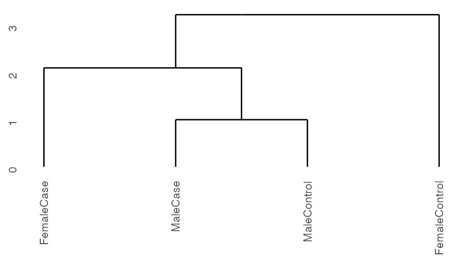
Running with cohorts and controls
When running with cohorts, K2Taxonomer includes the option of treating one of the levels within the cohorts variable as a control by specifying this value in the vehicle argument. In doing so, the values of each of the other cohorts will be evaluated in relation to this value.
## Run pre-processing
K2res <- K2preproc(sample.ExpressionSet,
                cohorts="group",
                vehicle="FemaleControl")
#> Collapsing group-level values with LIMMA.

## Cluster the data
K2res <- K2tax(K2res)

## Create dendrogram
dendro <- K2dendro(K2res)
ggdendrogram(dendro)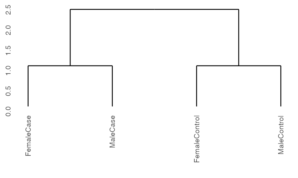
Differential analysis with controls
By specifying a control value, K2Taxonomer is able to assess directionality to differential analyses in relation to the control group, assigning direction of test statistics and gene assignments based on the subgroup in which the difference of the mean is more significantly different from the control group.
## Run DGE
K2res <- runDGEmods(K2res)

## Get differential results for one partition
head(K2results(K2res)$A$dge)
#>         gene        coef      mean         t         pval        fdr         B
#> 1   31328_at    48.56717  129.8394  4.676610 9.560191e-05 0.04780096 -3.663824
#> 2 31535_i_at    86.65559  266.8695  3.793490 8.923576e-04 0.22308941 -3.888946
#> 3   31471_at    55.86890  214.0319  3.491058 1.893595e-03 0.26321784 -3.972017
#> 4 31396_r_at  -479.16461 2504.3938 -3.424283 2.232095e-03 0.26321784 -4.594522
#> 5   31505_at -1438.84067 3404.9565 -3.357050 2.632178e-03 0.26321784 -4.009510
#> 6   31573_at   782.24198 2034.8062  3.099066 4.917064e-03 0.40163877 -4.594610
#>   edge
#> 1    2
#> 2    2
#> 3    2
#> 4    1
#> 5    2
#> 6    1

## Concatenate all results and generate table
DGEtable <- getDGETable(K2res)
head(DGEtable)
#>         gene        coef      mean         t         pval        fdr         B
#> 1   31328_at    48.56717  129.8394  4.676610 9.560191e-05 0.04780096 -3.663824
#> 2 31535_i_at    86.65559  266.8695  3.793490 8.923576e-04 0.22308941 -3.888946
#> 3   31471_at    55.86890  214.0319  3.491058 1.893595e-03 0.26321784 -3.972017
#> 4 31396_r_at  -479.16461 2504.3938 -3.424283 2.232095e-03 0.26321784 -4.594522
#> 5   31505_at -1438.84067 3404.9565 -3.357050 2.632178e-03 0.26321784 -4.009510
#> 6   31573_at   782.24198 2034.8062  3.099066 4.917064e-03 0.40163877 -4.594610
#>   edge node direction
#> 1    2    A        up
#> 2    2    A        up
#> 3    2    A        up
#> 4    1    A      down
#> 5    2    A      down
#> 6    1    A        up
Gene set analysis with controls
Accordingly, K2Taxonomer can now establish sets of genes that are both up- and down-regulated within a specific subgroup. We can now perform hyperenrichment with these additional gene sets.
## Run gene set hyperenrichment
K2res <- runGSEmods(K2res,
                    genesets=genesetsMadeUp,
                    qthresh=0.1)
Finally, differential analysis of single-sample gene set enrichment scores is performed in the same fashion as with differential analysis of gene expression, assessing directionality of differences in enrichment scores based on comparisons to the assigned control group.
## Create expression matrix with ssGSEA(GSVA) estimates
K2res <- runGSVAmods(K2res,
                    ssGSEAalg="gsva",
                    ssGSEAcores=1,
                    verbose=FALSE)

## Run differential analysis on enrichment score Expression Set
K2res <- runDSSEmods(K2res)

## Extract table of all hyper and sample-level enrichment tests
K2enrRes <- getEnrichmentTable(K2res)
head(K2enrRes)
#>   category node edge direction pval_hyper fdr_hyper nhits ndrawn ncats  ntot
#> 1      GS2    A    2        up     0.0025    0.0075     1      1    50 20000
#> 2      GS1    A    2        up     1.0000    1.0000     0      1    50 20000
#> 3      GS3    A    2        up     1.0000    1.0000     0      1    50 20000
#> 4      GS1    A    1        up         NA        NA    NA     NA    NA    NA
#>   pval_limma  fdr_limma      coef        mean        t         B     hits
#> 1 0.02901329 0.08703988 0.2336952 0.012747508 2.229860 -3.520723 31328_at
#> 2         NA         NA        NA          NA       NA        NA
#> 3 0.27895811 0.27895811 0.1169170 0.002788223 1.091252 -5.127802
#> 4 0.09904208 0.14856312 0.1660105 0.003870370 1.672058 -4.224175     <NA>
Here, we see that, although not statistically significant (“fdr_limma”=0.25), the enrichment score of “GS2” deviated further from the control group in subgroup, “node”=“B”; “edge”=“2”, compared to subgroup, “node”=“B”; “edge”=“1”.
Missing values for hyperenrichment analysis indicated that no genes were assigned to these specific subgroups and direction combinations. Missing values for differential enrichment score analysis indicate that, while genes were assigned to these specific subgroups and direction combinations, the enrichment score of the gene set deviated further from control in the alternative subgroup for that partition.
Additional topics
Multiple hypothesis correction
For each of the four statistical testing steps: differential gene expression, gene set hyperenrichment, differential single-sample gene set enrichment, and phenotypic variable testing, multiple hypothesis correction is performed across the aggregate set of p-values across all partitions using the Benjamini-Hochberg FDR correction (Benjamini and Hochberg 1995). This correction is performed independently for each of the four testing steps.
Unsupported combinations of arguments
-
vehicle != NULL with featMetric=“F” or recalcDataMatrix=TRUE
- Associations between the control cohort and remaining cohorts are generated prior to recursive partitioning. Either of these two argument specifications recalculate cohort-level statistics at each partition, many of which will not include the control cohort.
-
covariates != NULL with featMetric=“F” or recalcDataMatrix=TRUE
- Adjustments of gene expression values for covariates is performed prior to recursive partitioning. Either of these two argument specifications recalculate cohort-level statistics at each partition, some of which will not will not have any variation of this one or more of the covariates.
-
cohorts != NULL with infoClass != NULL
- Due to additional statistical and computational considerations for modeling data cohort-level information, currently phenotypic variable testing can only be performed for observation-level analysis.
References
Benjamini, Yoav, and Yosef Hochberg. 1995. “Controlling the False Discovery Rate: A Practical and Powerful Approach to Multiple Testing.” Journal of the Royal Statistical Society: Series B (Methodological) 57 (1): 289–300. https://doi.org/10.1111/j.2517-6161.1995.tb02031.x.
Hanzelmann, Sonja, Robert Castelo, and Justin Guinney. 2013. “GSVA: Gene Set Variation Analysis for Microarray and RNA-Seq Data.” BMC Bioinformatics 14 (1): 7. https://doi.org/10.1186/1471-2105-14-7.
Reed, Eric R., and Stefano Monti. 2020. “Multi-Resolution Characterization of Molecular Taxonomies in Bulk and Single-Cell Transcriptomics Data.” Preprint. Bioinformatics. https://doi.org/10.1101/2020.11.05.370197.
Ritchie, Matthew E., Belinda Phipson, Di Wu, Yifang Hu, Charity W. Law, Wei Shi, and Gordon K. Smyth. 2015. “Limma Powers Differential Expression Analyses for RNA-Sequencing and Microarray Studies.” Nucleic Acids Research 43 (7): e47–e47. https://doi.org/10.1093/nar/gkv007.