Running K2Taxonomer on Bulk Expression Data

Eric R. Reed

March 25, 2025

Introduction

This vignette describes the workflow for running K2Taxonomer recursive partitioning on bulk gene expression data (Reed and Monti 2021). Note, that many of these steps are shared with that of single-cell expression analyses. A vignette for running K2Taxonomer on single-cell expression data can be found here.

Requirements

Load packages

## K2Taxonomer package
library(K2Taxonomer)

## For example expression data
library(Biobase)

## For drawing dendrograms
library(ggdendro)

Read in sample ExpressionSet object

The main input of K2Taxonomer is an expression matrix object with approximately normally distributed expression values. Here we read in an example data set, which includes an expression matrix and sample data. See ?sample.ExpressionSet for more information about these data.

data(sample.ExpressionSet)

Running K2Taxonomer

Get necessary data objects

## Normalized expression matrix
expression_matrix <- exprs(sample.ExpressionSet)

## Sample information
sample_data <- pData(sample.ExpressionSet)

Create dummy example gene set object

genes <- unique(rownames(sample.ExpressionSet))
genesetsExample <- list(
    GS1=genes[1:50],
    GS2=genes[51:100],
    GS3=genes[101:150])

Initialize K2 object

The K2preproc() initializes the K2 object and runs pre-processing steps. Here, you can specify all arguments used throughout the analysis. Otherwise, you can specify these arguments within the specific functions for which they are implemented. See help pages for more information.

A description of arguments implemented in this vignette are

• object: “Expression Matrix”: Expression matrix to be used for partioning and downstram analyses.
• colData: “Data Frame”: A data frame which contains a row for each profile (i.e. columns in object).
• genesets: “Named List”: A named list of gene sets to be used for downstream annotation.

Note, that many of the default arguments are chosen for the single-cell workflow. However, these will be replaced if the argument, cohort is not specified, and a message is printed.

## Run pre-processing
K2res <- K2preproc(expression_matrix,
                   colData = sample_data,
                   genesets = genesetsExample)
#> No cohorts specified and clustFunc = 'cKmeansDownsampleSqrt' . Setting clustFunc = 'hclustWrapper'
#> No cohorts specified and recalcDataMatrix = TRUE. Setting recalcDataMatrix = FALSE
#> No cohorts specified and featMetric = 'F'. Setting featMetric = 'mad'

Perform recursive partitioning

The K2Taxonomer is run by K2tax(). At each recursion of the algorithm, the observations are partitioned into two sub-groups based on a compilation of repeated K=2 clustering on bootstrapped sampling of features. For each partition in the recursion, a stability metric is used to estimate robustness, which takes on values between 0 and 1, where values close to 1 represent the instance in which the same clustering occured in every or nearly every perturbation of a large set of observations. As the number of observations decreasing down the taxonomy the largest possible stability estimate decreases, such that the largest possible stability estimate of triplets and duplets, is 0.67 and 0.50, respectively.

The parameter, stabThresh, controls the minimum value of the stability metric to continue partitioning the observations. By default, stabThresh is set to 0, which will run the algorithm until until all observations fall into singlets. If we set stabThresh=0.5 the algorithm can not separate duplets, as well as larger sets that demonstrate poor stability when a partition is attempted. This can also be set during initialization with K2preproc().

Choosing an appropriate threshold is dependent on the size of the original data set. For large data sets, choosing small values will greatly increase runtime, and values between 0.8 and 0.7, are generally recommended.

## Run K2Taxonomer aglorithm
K2res <- K2tax(K2res,
               stabThresh=0.5)

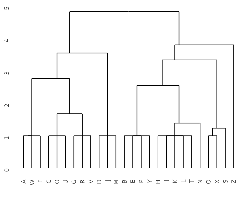
Generate dendrogram from K2Taxonomer results

Static dendrogram

## Get dendrogram from K2Taxonomer
dendro <- K2dendro(K2res)

## Plot dendrogram
ggdendrogram(dendro)

Interactive dendrogram

K2visNetwork(K2res)

Annotate K2Taxonomer results

Partition-level Differential Gene Expression Analysis

K2res <- runDGEmods(K2res)
#> Running DGE for partition:
#>   1 / 10 
#>   2 / 10 
#>   3 / 10 
#>   4 / 10 
#>   5 / 10 
#>   6 / 10 
#>   7 / 10 
#>   8 / 10 
#>   9 / 10 
#>   10 / 10

Perform gene set based analyses

### Perform Fisher Exact Test based over-representation analysis
K2res <- runFISHERmods(K2res)

### Perform single-sample gene set scoring
K2res <- runScoreGeneSets(K2res)
#> Scoring gene sets with GSVA.
#> Estimating GSVA scores for 3 gene sets.
#> Estimating ECDFs with Gaussian kernels

### Perform partition-evels differential gene set score analysis
K2res <- runDSSEmods(K2res)
#> Running different enrichment score for partition:
#>   1 / 10 
#>   2 / 10 
#>   3 / 10 
#>   4 / 10 
#>   5 / 10 
#>   6 / 10 
#>   7 / 10 
#>   8 / 10 
#>   9 / 10 
#>   10 / 10

Explore Annotation Results

Partition-level Differential Gene Expression Analysis

Create Static Table of DGE Results

DGEtable <- getDGETable(K2res)
head(DGEtable)
#>       gene      coef      mean        t       df         pval          fdr edge
#> 1 31583_at 1444.0457 2819.3481 7.090895 27.31219 1.184936e-07 0.0003465938    2
#> 2 31546_at 1180.8349 1963.0257 7.019826 27.31219 1.419856e-07 0.0004151659    2
#> 3 31527_at 1579.2611 3428.9188 6.704309 27.31219 3.191638e-07 0.0009329158    2
#> 4 31568_at 1372.3639 2866.9177 6.494425 27.31219 5.503484e-07 0.0016081181    2
#> 5 31573_at 1155.9527 2034.8062 6.331862 27.31219 8.418968e-07 0.0024591805    2
#> 6 31492_at  267.2776  307.9889 6.314658 27.31219 8.807715e-07 0.0025718527    2
#>   node direction
#> 1    A        up
#> 2    A        up
#> 3    A        up
#> 4    A        up
#> 5    A        up
#> 6    A        up

Create Interactive Table of DGE Results

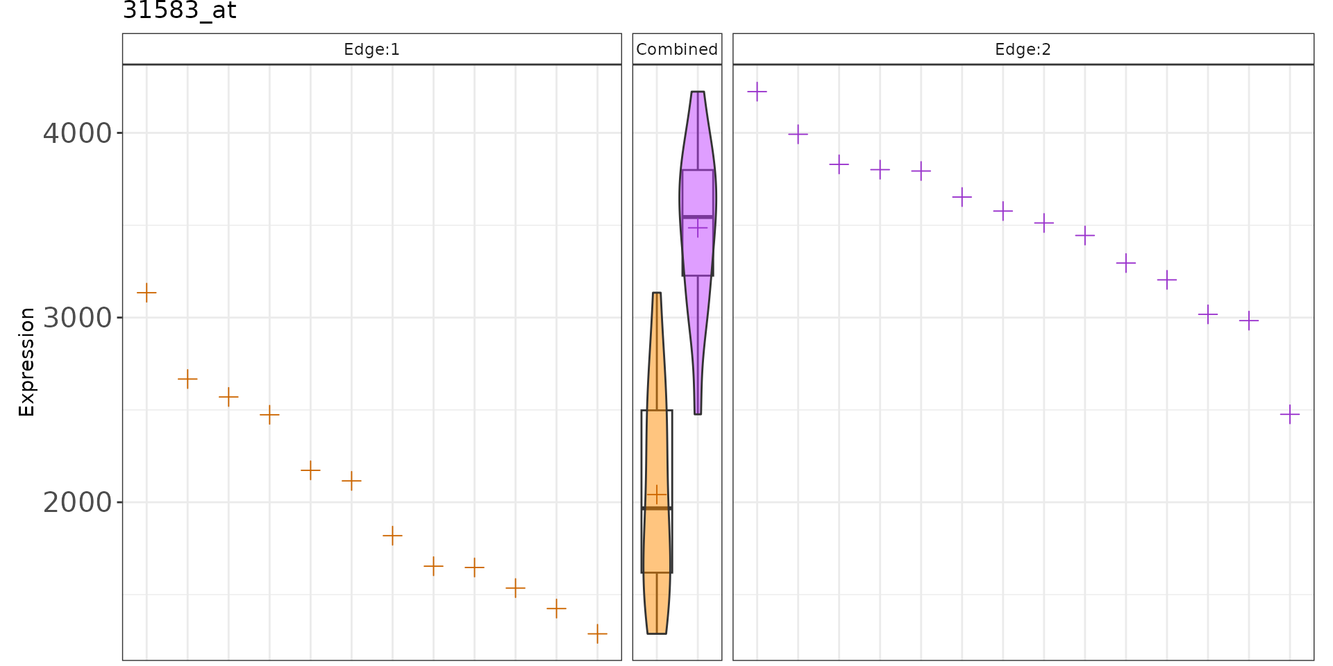
getDGEInter(K2res, minDiff = 1, node = c("A"), pagelength = 10)

Create Plot of Gene Expression

plotGenePathway(K2res, feature = "31583_at", node = "A", subsample = FALSE)
#> K2eMatDS() is empty, using K2eMat() instead

Create Static Plot Gene Expression

plotGenePathway(K2res, feature = "31583_at", node = "A", use_plotly = FALSE)
#> K2eMatDS() is empty, using K2eMat() instead

Partition-level Gene Set Enrichment Results

Create Static Table of Gene Set Results

ENRtable <- getEnrichmentTable(K2res)
head(ENRtable)
#>   category node edge direction pval_fisher fdr_fisher nhits ndrawn ncats  ntot
#> 1      GS1    G    2        up          NA         NA    NA     NA    NA    NA
#> 2      GS3    A    1        up          NA         NA    NA     NA    NA    NA
#> 3      GS1    A    1        up          NA         NA    NA     NA    NA    NA
#> 4      GS3    G    2        up          NA         NA    NA     NA    NA    NA
#> 5      GS1    B    1        up          NA         NA    NA     NA    NA    NA
#> 6      GS1    E    2        up           1          1     0      1    50 20000
#>    pval_limma  fdr_limma      coef         mean        t hits
#> 1 0.004463359 0.08034045 0.3012940  0.171766848 3.954464 <NA>
#> 2 0.004788253 0.08140029 0.1851625  0.008112864 2.985053 <NA>
#> 3 0.009477649 0.15164239 0.1956683 -0.001944512 2.723717 <NA>
#> 4 0.081900911 1.00000000 0.2107563  0.112850770 1.997425 <NA>
#> 5 0.130129246 1.00000000 0.2138517  0.103415335 1.563280 <NA>
#> 6 0.179713417 1.00000000 0.1191463 -0.100852195 1.370722

Create Interactive Table of Gene Set Results

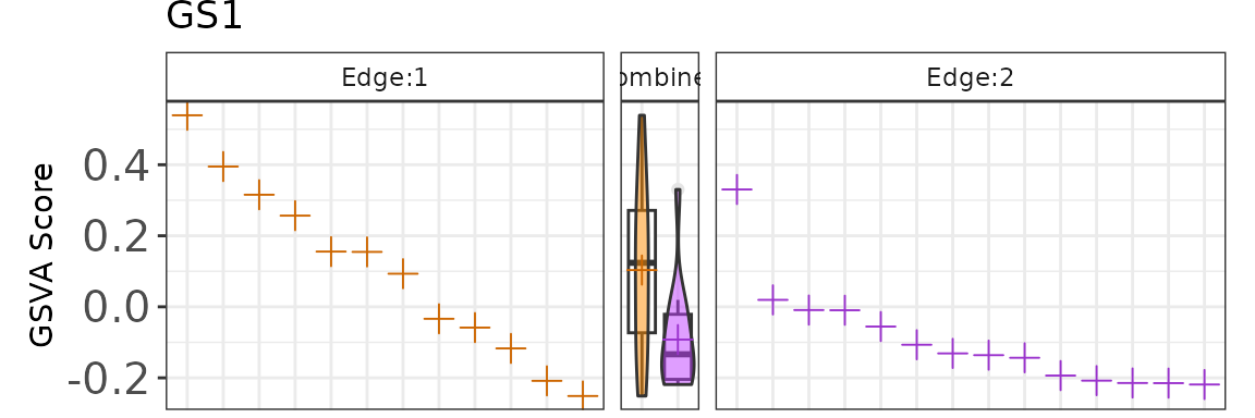
getEnrichmentInter(K2res, nodes = c("A"), pagelength = 10)

Create Interactive Plot of Single-sample Scoring

plotGenePathway(K2res, feature = "GS1", node = "A", type = "gMat")

Create Static Plot of Single-sample Scoring

plotGenePathway(K2res, feature = "GS1", node = "A", type = "gMat", use_plotly = FALSE)

Create Dashboard

For more information about K2Taxonomer dashboards, read this vignette.

# Not run
K2dashboard(K2res, "K2results_sample.ExpressionSet")

Implementation Options

Parellel excecutation

The K2Taxonomer workflow can take a long time with large data sets. Accordingly, it is generally recommended to run the workflow using parallel computing. This can be implemented easily by setting the useCors argument in K2preproc()

# Not run
K2res <- K2preproc(expression_matrix,
                   colData = sample_data,
                   genesets = genesetsExample,
                   stabThresh=0.5,
                   useCors = 8) ## Runs K2Taxonomer in parellel with eight cores.

Using ExpresssionSet object directly

In addition to expression matrices, ExpressionSet objects may be input directly with the object argument. When implemented, colData isn’t specified and this information is pulled from the phenotype data of the ExpressionSet object.

K2res_eSet <- K2preproc(sample.ExpressionSet,
                   genesets = genesetsExample,
                   stabThresh=0.5)
#> No cohorts specified and clustFunc = 'cKmeansDownsampleSqrt' . Setting clustFunc = 'hclustWrapper'
#> No cohorts specified and recalcDataMatrix = TRUE. Setting recalcDataMatrix = FALSE
#> No cohorts specified and featMetric = 'F'. Setting featMetric = 'mad'

## Run recursive partitioning algorithm
K2res_eSet <- K2tax(K2res_eSet)

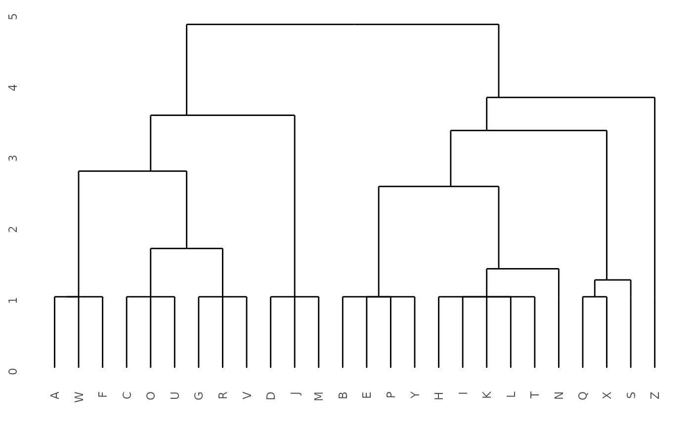
## Get dendrogram from K2Taxonomer
dendro_eSet <- K2dendro(K2res_eSet)

## Plot dendrogram
ggdendrogram(dendro_eSet)

References

Reed, Eric R., and Stefano Monti. 2021. “Multi-Resolution Characterization of Molecular Taxonomies in Bulk and Single-Cell Transcriptomics Data.” Nucleic Acids Research. https://doi.org/10.1093/nar/gkab552.