Clustering of Real Data: the Drug Matrix
We will use the DrugMatrix subset previously described for our examples. This data corresponds to chemical perturbation experiments, whereby rats are exposed to different chemicals, and their liver's RNA is profiled.
We upload the data and perform a drastic variation filtering to obtain a small and easy to manage dataset.
data(dm10)

DM <- variationFilter(dm10,ngenes=1000,do.plot=TRUE,verbose=FALSE)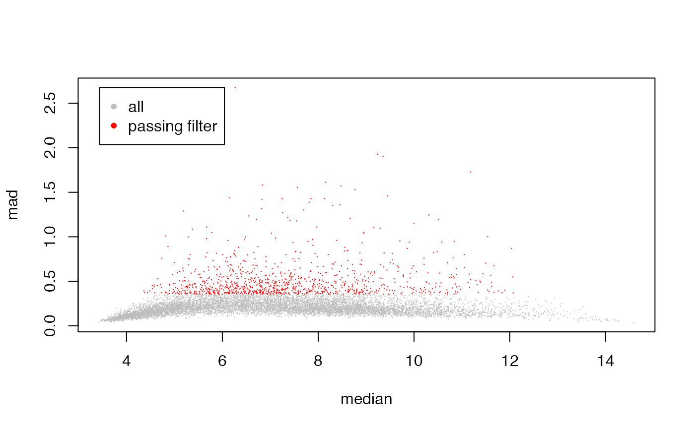
Hierarchical Clustering
Let us analyze the data by carrying out hierarchical clustering. We'll use heatmap.plus to visualize the data. Let us first define a simple function to create a color gradient to be used for coloring the gene expression heatmaps.
colGradient <- function( cols, length, cmax=255 )
{
## e.g., to create a white-to-red gradient with 10 levels
##
## colGradient(cols=c('white','red'),length=10)
##
## or, to create a blue-to-white-to-red gradients with 9 colors (4 blue's, white, 4 red's)
##
## colGradient(cols=c('blue','white','red'),length=9)
##
ramp <- colorRamp(cols)
rgb( ramp(seq(0,1,length=length)), max=cmax )
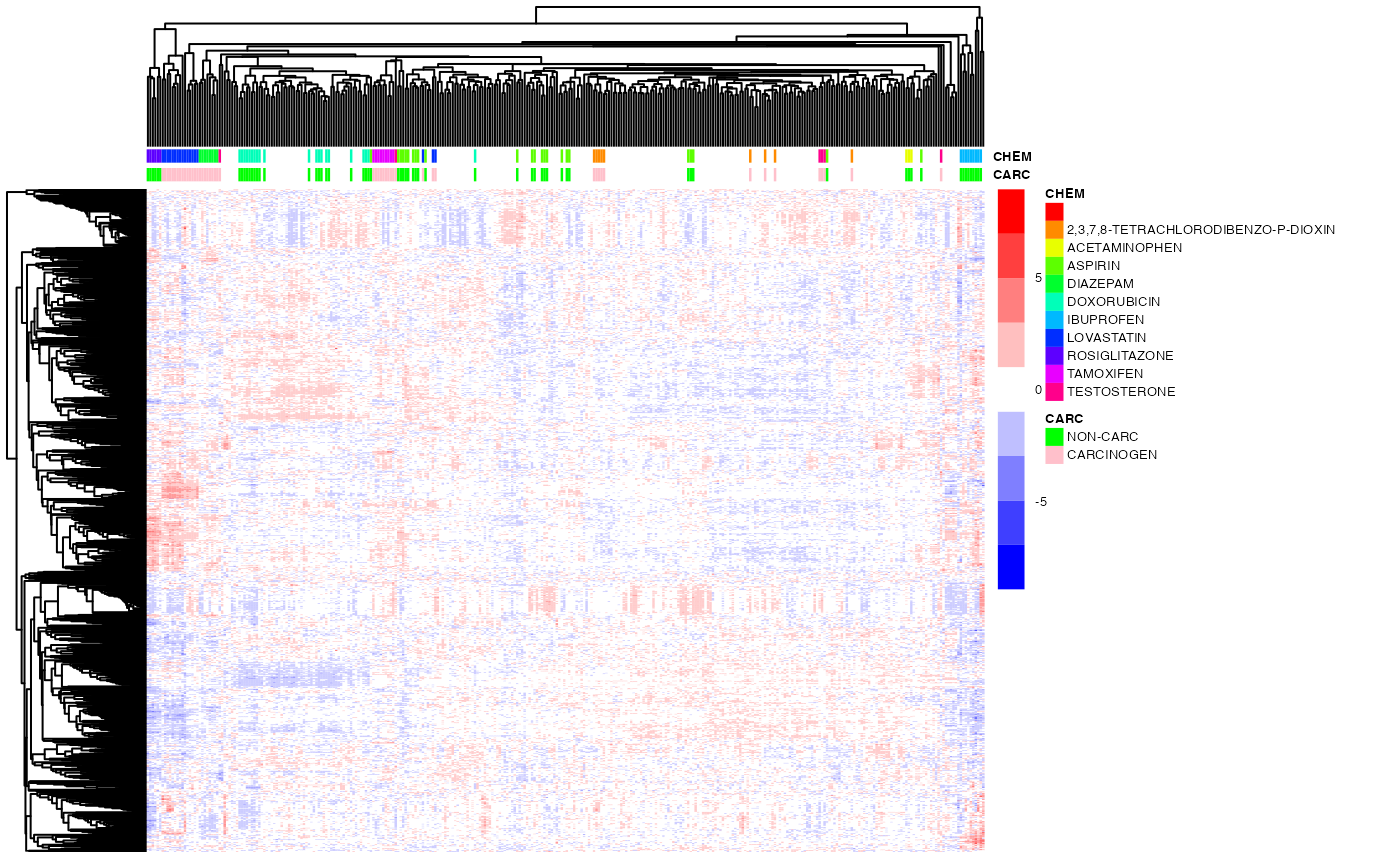
}Next, let us perform the actual clustering. While the function heatmap.plus can carry out hierarchical clustering internally, we explicitely call hclust outside the function call to illustrate its use (this will also save computation time should one want to call heatmap.plus multiple times with different color coding or other changes that would not affect the clustering).
Notice that the heatmap color is somewhat saturated. In the module R/Heatmaps.Rmd we present additional visualization functions that do a better job at color-coding the heatmap.
chemicals <- unique(pData(dm10)[,"CHEMICAL"])
annot <- data.frame(CARC=dm10$Carcinogen_liv,
                    CHEM=dm10$CHEMICAL,
                    row.names = Biobase::sampleNames(dm10))
annot_col <- list(
    CARC=c("NON-CARC"="green","CARCINOGEN"="pink"),
    CHEM=data.frame(chem=chemicals,cols=rainbow(length(chemicals))) %>% tibble::deframe())

## color gradient for the expression levels (blue=down-regulated; white=neutral; red=up-regulated)
bwrPalette <- colGradient(c("blue","white","red"),length=9)

## cluster rows (genes) and columns (samples)
hc_row <- hclust(as.dist(1-cor(t(exprs(DM)))),method="ward.D2") # genes by correlation
hc_col <- hclust(dist(t(exprs(DM))),method="ward.D2")           # samples by euclidean distance (default)

pheatmap(exprs(DM),
         color=bwrPalette,
         annotation_col = annot,
         annotation_colors = annot_col,
         cluster_rows=hc_row,
         cluster_cols=hc_col,
         show_rownames = FALSE,
         show_colnames = FALSE,
         scale = "row",
         fontsize = 5)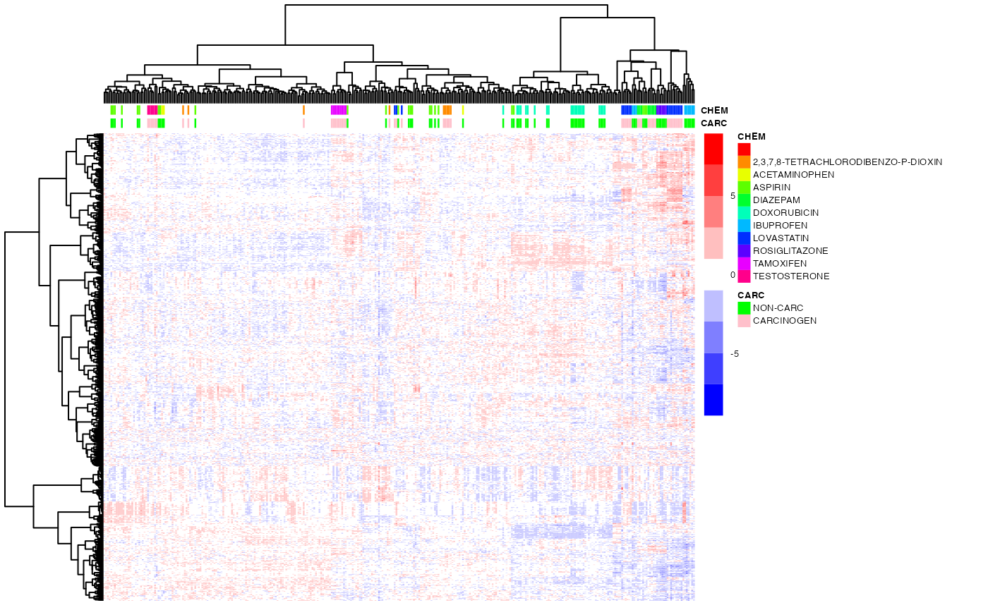
## color coding of the samples indicating carcinogenicity status and chemical
chemicals <- unique(pData(dm10)[,"CHEMICAL"])
CSC <- cbind(CARC=c("white","green","pink")[match(pData(dm10)[,"Carcinogen_liv"],c(NA,"NON-CARC","CARCINOGEN"))],
             CHEM=rainbow(length(chemicals))[match(pData(dm10)[,"CHEMICAL"],chemicals)])

## color gradient for the expression levels (blue=down-regulated; white=neutral; red=up-regulated)
bwrPalette <- colGradient(c("blue","white","red"),length=13)

## cluster rows (genes) and columns (samples)
hc.row <- hclust(as.dist(1-cor(t(exprs(DM)))),method="ward.D2") # genes by correlation
hc.col <- hclust(dist(t(exprs(DM))),method="ward.D2")           # samples by euclidean distance (default)

## draw the heatmap (hide row and col labels since they'd be unreadable)
heatmap.plus(exprs(DM),
             Rowv=as.dendrogram(hc.row),
             Colv=as.dendrogram(hc.col),
             col=bwrPalette,
             ColSideColors=CSC,
             labCol=NA,labRow=NA)
pheatmap(DM)
Optimal Leaf Ordering
As discussed in class, hierarchical clustering induces a partial ordering of the dendogram leaves (i.e., of the clustered items), modulo the 'flipping' of any of the sub-trees. However, one can obtain a total ordering by using the leaf-ordering algorithm developed by Bar-Joseph et al. (2001), which minimizes the distance betwees adjacent items in two distinct sub-trees.
library(cba) # load the necessary pacakge

## First, call hclust, then call the leaf-ordering algorithm and re-order the dendrogram

hc_col <- hclust(dist(t(exprs(DM))),method="ward.D2")
ord <- order.optimal(dist(t(exprs(DM))),merge=hc_col$merge)
hc_col$merge <- ord$merge
hc_col$order <- ord$order

## visualize the results (and compare, visually, to the results w/o optimal leaf ordering above)
pheatmap(exprs(DM),
         color=bwrPalette,
         annotation_col = annot,
         annotation_colors = annot_col,
         cluster_rows=hc_row,
         cluster_cols=hc_col,
         show_rownames = FALSE,
         show_colnames = FALSE,
         scale = "row",
         fontsize = 5)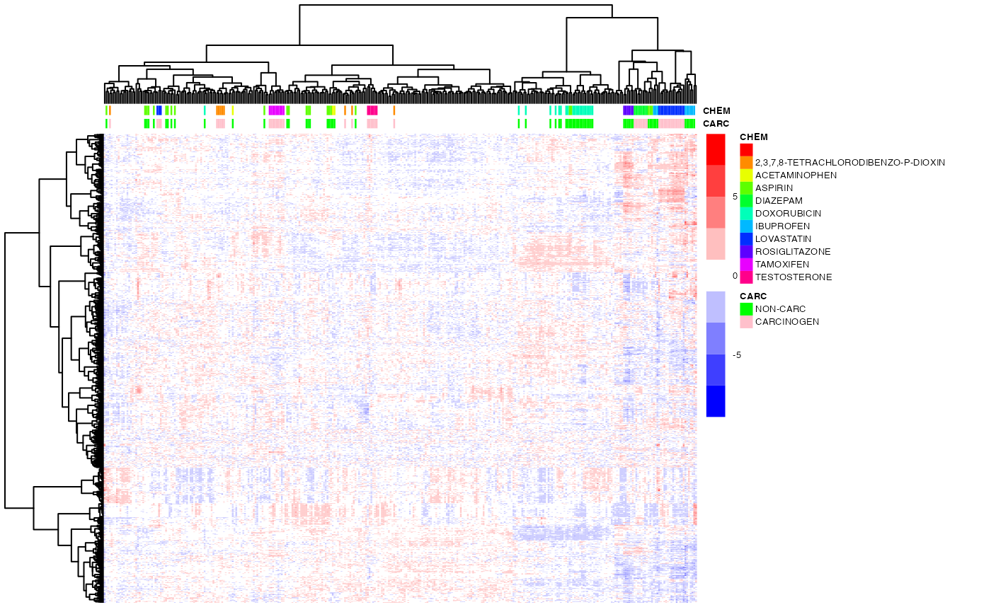
## since this is a step always worth performing, let's define a simple function that implements the necessary steps
hcopt <- function(d, HC=NULL, method = "ward.D", members = NULL)
{
  if ( is.null(HC) ) {
    HC <- hclust(d,method=method,members=members)
  }
  ORD <- order.optimal(d,merge=HC$merge)
  HC$merge <- ORD$merge
  HC$order <- ORD$order
  HC
}
## ok, now we can easily use the function in place of hclust
ho_row <- hcopt(as.dist(1-cor(t(exprs(DM)))),method="ward.D2") # genes by correlation
ho_col <- hcopt(dist(t(exprs(DM))),method="ward.D2")            # samples by euclidean distance (default)
pheatmap(exprs(DM),
         color=bwrPalette,
         annotation_col = annot,
         annotation_colors = annot_col,
         cluster_rows=ho_row,
         cluster_cols=ho_col,
         show_rownames = FALSE,
         show_colnames = FALSE,
         scale = "row",
         fontsize = 5)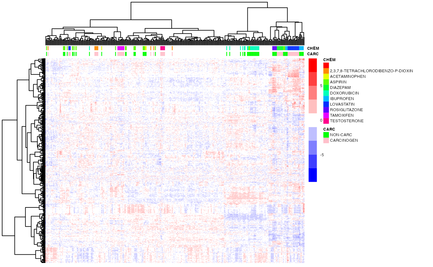
Alternative Agglomeration Rules
In the examples above, we used the Ward method as our agglomeration rule. One of the nice properties of Ward is that it tends to yield well-balanced trees. Let us not look at alternative agglomeration rules.
## complete linkage
ho_row1 <- hcopt(as.dist(1-cor(t(exprs(DM)))),method="complete") # genes by correlation
ho_col1 <- hcopt(dist(t(exprs(DM))),method="complete")           # samples by euclidean distance (default)
pheatmap(exprs(DM),
         color=bwrPalette,
         annotation_col = annot,
         annotation_colors = annot_col,
         cluster_rows=ho_row1,
         cluster_cols=ho_col1,
         show_rownames = FALSE,
         show_colnames = FALSE,
         scale = "row",
         fontsize = 5)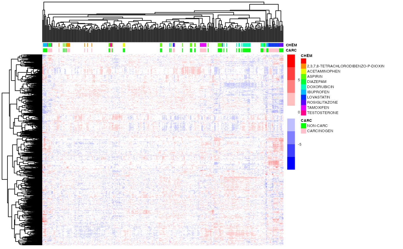
## single linkage
ho_row2 <- hclust(as.dist(1-cor(t(exprs(DM)))),method="single") # genes by correlation
ho_col2 <- hcopt(dist(t(exprs(DM))),method="single")            # samples by euclidean distance (default)
pheatmap(exprs(DM),
         color=bwrPalette,
         annotation_col = annot,
         annotation_colors = annot_col,
         cluster_rows=ho_row2,
         cluster_cols=ho_col2,
         show_rownames = FALSE,
         show_colnames = FALSE,
         scale = "row",
         fontsize = 5)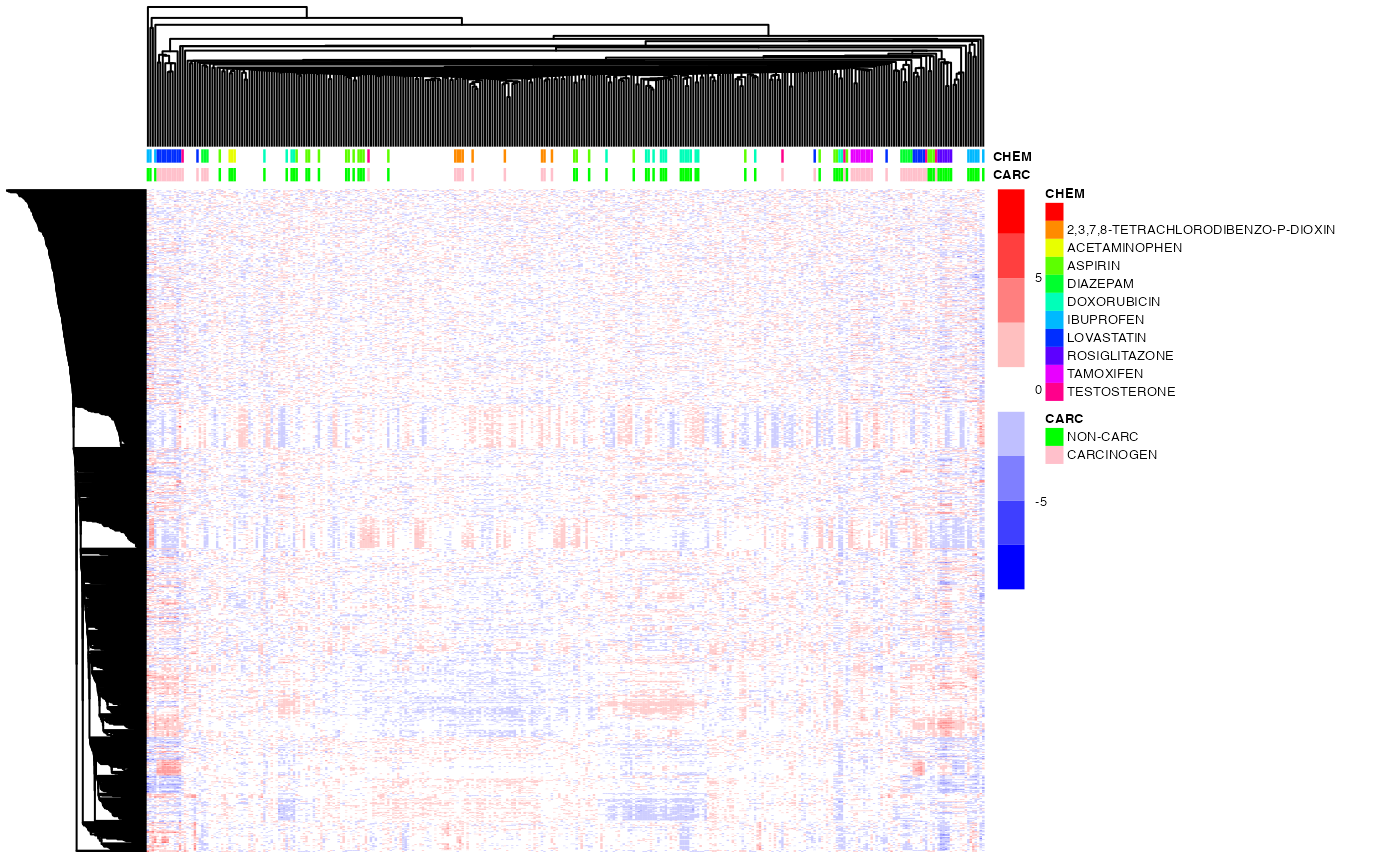
## average linkage
ho_row3 <- hclust(as.dist(1-cor(t(exprs(DM)))),method="average") # genes by correlation
ho_col3 <- hcopt(dist(t(exprs(DM))),method="average")            # samples by euclidean distance (default)
pheatmap(exprs(DM),
         color=bwrPalette,
         annotation_col = annot,
         annotation_colors = annot_col,
         cluster_rows=ho_row3,
         cluster_cols=ho_col3,
         show_rownames = FALSE,
         show_colnames = FALSE,
         scale = "row",
         fontsize = 5)