Linear Regression

This is a simple example, where we generate data from a given linear model (with known intercept and slope), and then we apply linear regression to estimate the parameters of the data generating model.

set.seed(159) # for reproducible results 
nobs <- 1000   # sample size
beta0 <- 1     # true intercept
beta1 <- 0.15  # true slope
## simulate an imaginary dependent variable (e.g., age between 15-75)
X <- sample(15:75,nobs,replace=TRUE)
Y <- rnorm(nobs,mean=beta0 + beta1 * X,sd=1)

## or, equivalently
## Y <- beta0 + beta1 * X + rnorm(nobs,mean=0,sd=1)

## png(file.path(OMPATH,"Rmodules/figures/diffanalLM.png"))
par(mar=c(c(5, 4, 4, 5) + 0.1))
plot(X,Y,pch=20,xlab="age",ylab="expression")
abline(beta0,beta1,col="red",lty=3,lwd=2)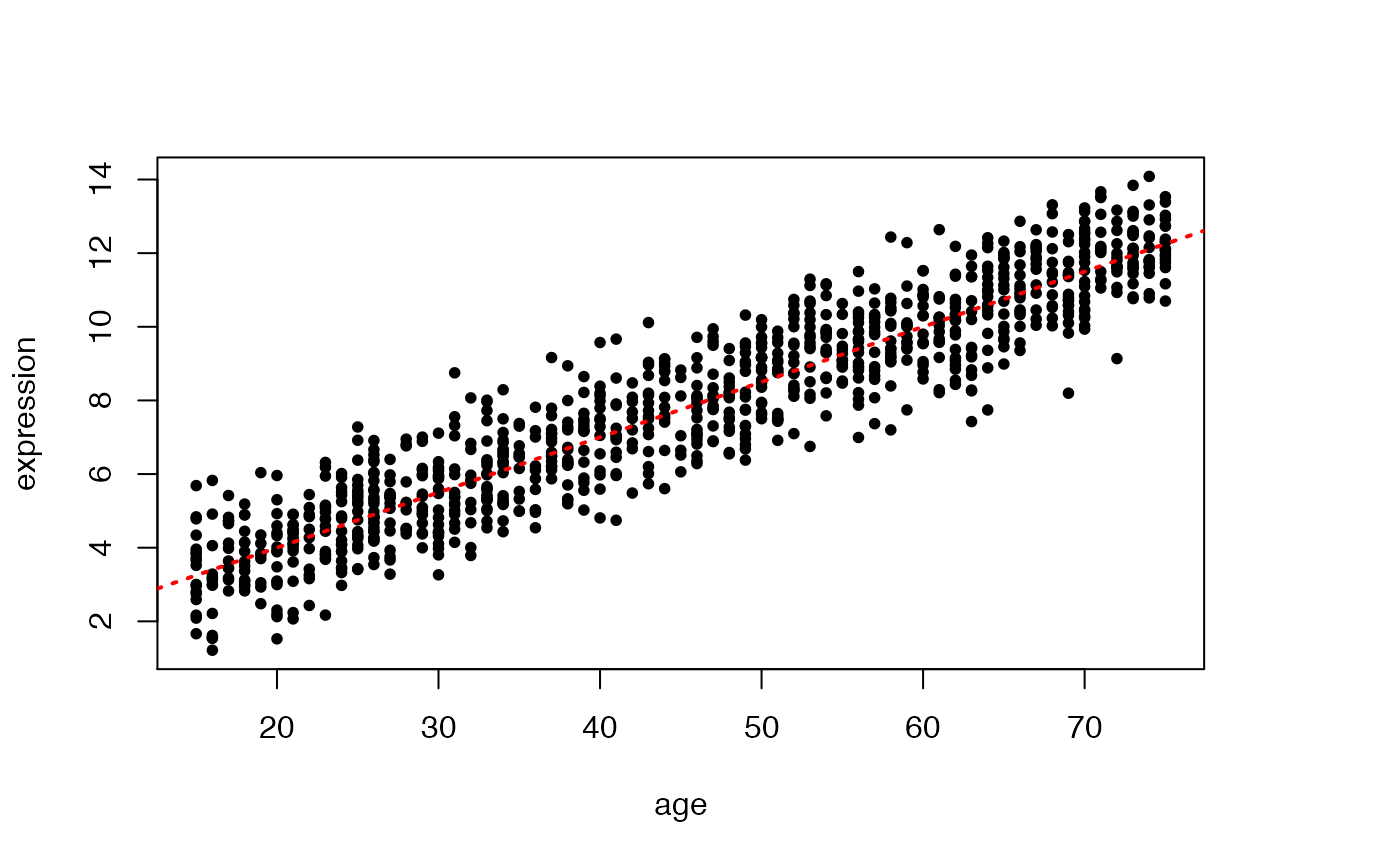

## notice the use of 'expression' to display mathematical symbols
##text(50,2,labels=expression(Y=beta[0]+beta[1]*X),las=1)

We now fit a linear model to the generated data by lm.

LM <- lm(Y ~ X)
print(summary(LM))

## 
## Call:
## lm(formula = Y ~ X)
## 
## Residuals:
##     Min      1Q  Median      3Q     Max 
## -3.2064 -0.6992 -0.0125  0.6870  3.0741 
## 
## Coefficients:
##             Estimate Std. Error t value Pr(>|t|)    
## (Intercept) 1.004106   0.088484   11.35   <2e-16 ***
## X           0.150705   0.001812   83.18   <2e-16 ***
## ---
## Signif. codes:  0 '***' 0.001 '**' 0.01 '*' 0.05 '.' 0.1 ' ' 1
## 
## Residual standard error: 1.014 on 998 degrees of freedom
## Multiple R-squared:  0.8739, Adjusted R-squared:  0.8738 
## F-statistic:  6919 on 1 and 998 DF,  p-value: < 2.2e-16

As you can see, the estimates are quite close to the generating parameters.

Stefano Monti