Geneset projection based on ASSIGN

In this module, we illustrate the use of a method of pathway (or geneset, or signature) projection. In particular, we show an example of use of Adaptive Signature Selection and InteGratioN (ASSIGN). See Rmodule_GeneSetProjectionGSVA and Rmodule_KSenrichment for an example of alternative method of pathway projection based on KS enrichment.

We start by loading the ASSIGN package, available through Bioconductor, and by sourcing a wrapper script for its easier handling.

library(BS831)
library(Biobase)      # the package with the ExpressionSet definition, among others
library(ASSIGN)       # the assign package
library(RColorBrewer) # for heatmap visualization

We next load the necessary data, consisting of gene expression profiles from the TCGA head and neck squamous carcinoma (HNSC) dataset, and a signature corresponding to combined shRNA knockdown of TAZ and YAP, two transcriptional effectors of the hippo pathway.

data(HNSC_RNASeq_ES)

## load the GEP data
hnsc <- HNSC_RNASeq_ES
dim(hnsc)

## Features  Samples 
##    20263      566

## load the signature
sig <- read.delim(file.path(system.file("extdata", package="BS831"), "yap_taz.gmt"), header=F,stringsAsFactors=F,row.names=1 )
## show the signature (one per row)
rownames(sig)

## [1] "TAZ.YAP.UP" "TAZ.YAP.DN"

We will only project genes that go down upon YAP/TAZ knockdown for this example.

gene_set <- as.character(sig["TAZ.YAP.DN",])
gene_set <- gene_set[gene_set!=""] # Strip off any empty entries
print(length(gene_set))            # Show the size of the gene signature

## [1] 381

We are now ready to run ASSIGN. We specify the output directory where all ASSIGN output will be stored. This folder will automatically be created if it does not already exist.

set.seed(479) # for reproducible results
assign_out_dir <- file.path( tempdir(), "yap_taz_activated_HNSC" ) 
run_assign(ES = hnsc,eSig = gene_set, oDir = assign_out_dir, iter=3000)

## Running with signature:                   gene_set 
## Number of genes in signature:             381 
## Overlap between signature and ESet genes: 358 
## Run ASSIGN with mixture modelling beta:   TRUE  ..
## Saving output to directory:               /tmp/Rtmph0YdcH/yap_taz_activated_HNSC

## Done!

Load the generated ASSIGN output object and generate heatmaps to visualize the signature projection

load( file.path(assign_out_dir,"output.rda"))
plotAll(eSet = hnsc,output.data =output.data,title = "YAP/TAZ activation" ,gene_list =  gene_set)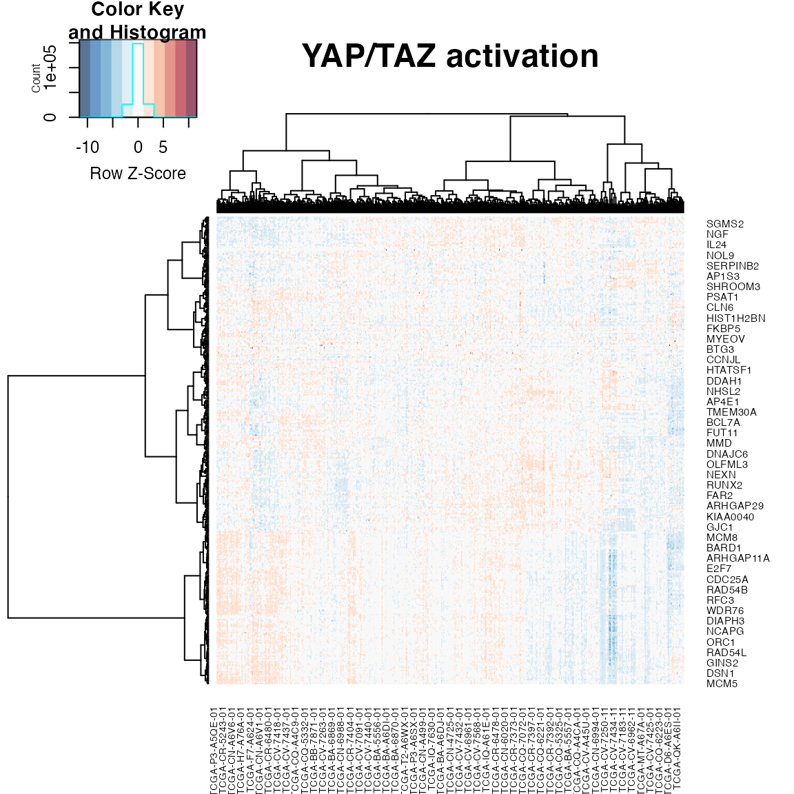

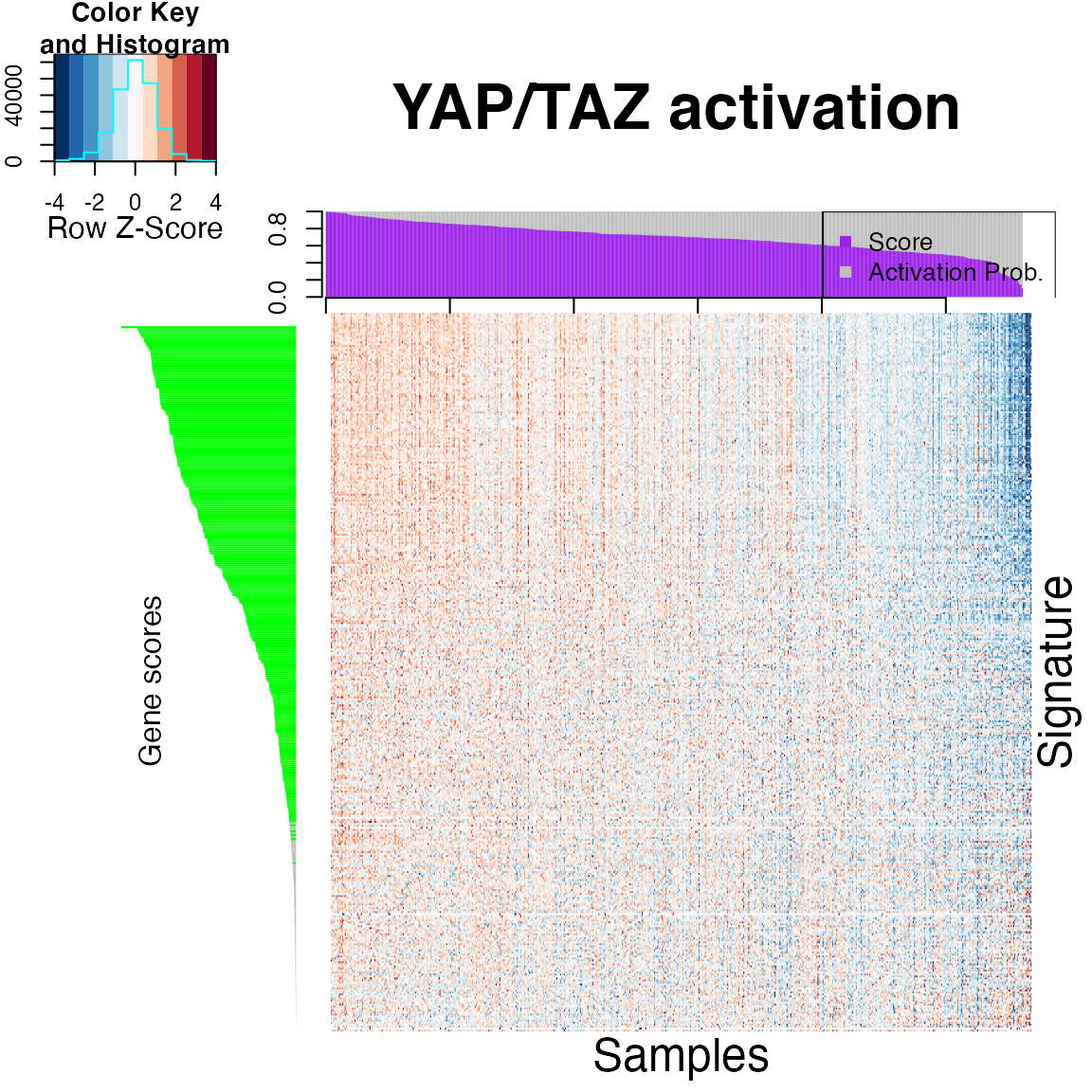
Geneset projection is particularly useful when we need to determine the activity of important proteins, like transcription factors (or effectors, more in general), which often is not properly captured by their transcript expression. In these cases, looking at the coordinated expression of their downstream targets is often more effective.

Let’s take a look at the gene expression profiles for YAP and TAZ with respect to tumor grade. Below, we show that while the expression of neither transcripts is significantly associated with grade progression, their activity as captured by the ASSIGN scores (i.e., by the coordinated expression of their downstream targets) is significantly associated in the epxected direction, with higher grades associated to higher TAZ/YAP activity.

We first fetch the expression values for the two genes. Note their specific gene symbols (YAP1 and WWTR1)

## YAP1 is the gene symbol for YAP
yap1 <- log2(as.numeric(exprs(hnsc)[fData(hnsc)$gene_symbol %in% "YAP1"]))
## WWTR1 is the gene symbol for TAZ
wwtr1<-log2(as.numeric(exprs(hnsc)[fData(hnsc)$gene_symbol %in% "WWTR1"]))

We next extract the generated ASSIGN YAP/TAZ projection scores for each sample.

scores_file <- file.path(assign_out_dir,"pathway_activity_testset.csv")
scores <- read.csv(scores_file,stringsAsFactors=F,header=T)
yap.taz.scores <- scores[,2]
summary(yap.taz.scores)

##    Min. 1st Qu.  Median    Mean 3rd Qu.    Max. 
##  0.0000  0.5850  0.7084  0.6881  0.8169  0.9973

We then make a data frame combinding the yap/taz ASSIGN scores, yap and taz gene expression and tumor grade. We will visualize these to see the effect of geneset projection vs single gene expression analysis

d <- data.frame("sample_ID"=scores[,1],
                "tumor_grade"=hnsc$my_grade,
                "assign_scores"=yap.taz.scores,
                "yap1"=yap1,
                "wwtr1"=wwtr1)

d <- d[!(d$tumor_grade %in% c(NA,"gx")),] # Remove samples with missing grade information (NA or "gx")
d$tumor_grade <- as.factor(as.character(d$tumor_grade)) # Remove eliminated entries

Plot individual gene expression values, as well as YAP/TAZ ASSIGN scores with respect to tumor grade

f <- grDevices::colorRampPalette(c("gray75","darkgreen"))
## Make a gradient of colours for different tumor grade
grade.cols <- f(length(table(as.character(d$tumor_grade)))) 

#par(mfrow=c(3,1)) #Arrange plots in single column
boxplot(yap1~tumor_grade,col=grade.cols,data = d,main="YAP gene expression \nwrt tumor grade")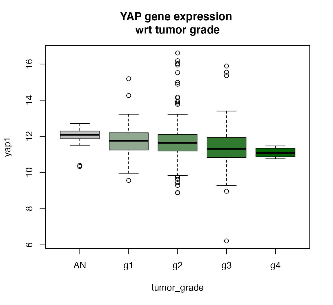

boxplot(wwtr1~tumor_grade,col=grade.cols,data = d,main="TAZ gene expression \nwrt tumor grade")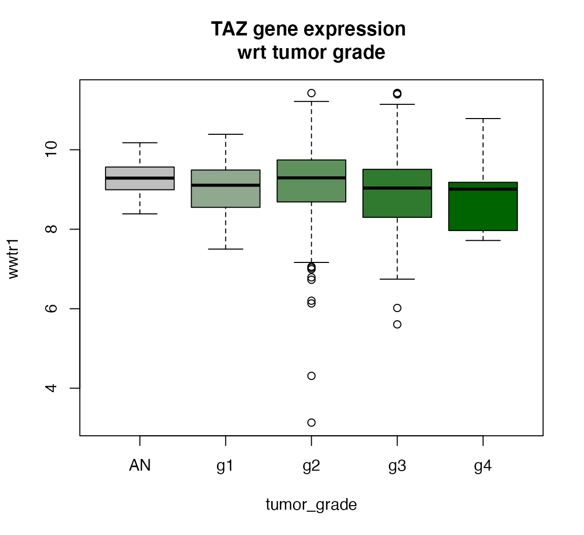

boxplot(assign_scores~tumor_grade,col=grade.cols,data=d,main="YAP/TAZ ASSIGN scores \nwrt tumor grade")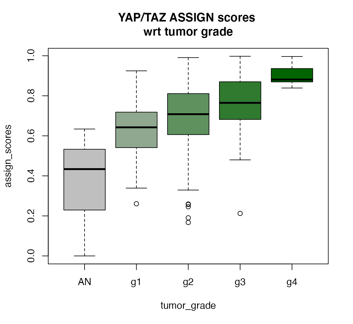

## association with TAZ/YAP "activity" highly significant
anova(lm(assign_scores~tumor_grade,data=d))

## Analysis of Variance Table
## 
## Response: assign_scores
##              Df  Sum Sq Mean Sq F value    Pr(>F)    
## tumor_grade   4  5.5282 1.38205  62.333 < 2.2e-16 ***
## Residuals   539 11.9508 0.02217                      
## ---
## Signif. codes:  0 '***' 0.001 '**' 0.01 '*' 0.05 '.' 0.1 ' ' 1

Stefano Monti