RNA-seq differential expression analysis with DEseq2, edgeR and limma
Amy Li, Eric Reed, Stefano Monti
Source:vignettes/docs/DiffanalysisRNAseqComparison.Rmd
DiffanalysisRNAseqComparison.RmdIn this module, we show application of different tools for differential analysis to count data from RNA-sequencing.
library(BS831)
library(Biobase)
library(limma)
library(edgeR)
library(DESeq2)
library(biomaRt)
library(VennDiagram)
Let’s start by writing wrapper functions for each tool. This is useful so as to have a go-to place where to be reminded of the sequences of commands needed to run a given tool.
print(run_deseq)## function(eset, class_id, control, treatment)
## {
## ## require(DESeq2)
## control_inds <- which(pData(eset)[, class_id] == control)
## treatment_inds <- which(pData(eset)[, class_id] == treatment)
## eset.compare <- eset[, c(control_inds, treatment_inds)]
##
## ## make deseq2 compliant dataset
## colData <- data.frame(condition=as.character(pData(eset.compare)[, class_id]))
## dds <- DESeqDataSetFromMatrix(exprs(eset.compare), colData, formula( ~ condition))
##
## ## set reference to control, otherwise default is alphabetical order
## dds$condition <- factor(dds$condition, levels=c(control,treatment))
##
## ## run deseq2
## ## 3 steps:
## ## 1. estimate size factors
## ## 2. estimate dispersion
## ## 3. negative binomial GLM fitting and wald test
## dds_res <- DESeq(dds)
## res <- results(dds_res)
## res$dispersion <- dispersions(dds_res)
## return(res)
## }
## <environment: namespace:BS831>
print(run_edgeR)## function(eset, class_id, control, treatment)
## {
## ##library(edgeR)
## control_inds <- which(pData(eset)[, class_id] == control)
## treatment_inds <- which(pData(eset)[, class_id] == treatment)
##
## ## make edgeR compliant dataset
## eset.compare <- eset[, c(control_inds, treatment_inds)]
## condition <- as.character(pData(eset.compare)[, class_id])
##
## ## run edgeR
## y <- DGEList(counts=exprs(eset.compare), group = condition)
## y <- calcNormFactors(y)
## y <- estimateGLMCommonDisp(y)
## y <- estimateGLMTrendedDisp(y)
## y <- estimateGLMTagwiseDisp(y)
## et <- exactTest(y)
## res <- topTags(et, n = nrow(eset.compare), sort.by = "none")
## return(res)
## }
## <environment: namespace:BS831>
print(run_limma)## function(eset, class_id, control, treatment)
## {
## control_inds <- which(pData(eset)[, class_id] == control)
## treatment_inds <- which(pData(eset)[, class_id] == treatment)
##
## eset.compare <- eset[, c(control_inds, treatment_inds)]
## condition <- as.character(pData(eset.compare)[, class_id])
## colData <- data.frame(condition=as.character(pData(eset.compare)[, class_id]))
##
## design <- model.matrix(~ 0 + factor(condition))
## colnames(design) <- levels( factor(condition))
## fit <- lmFit(eset.compare, design)
## command_str <- paste("makeContrasts(",
## "(", treatment , "-", control, ")",
## ",levels = design)", sep = "")
##
## contrast.matrix <- eval(parse(text=command_str))
## fit2 <- contrasts.fit(fit, contrast.matrix)
## fit2 <- eBayes(fit2)
## res <- topTable(fit2, coef=1, adjust="BH", sort.by = "none", number=Inf)
## return(res)
## }
## <environment: namespace:BS831>Loading zebrafish count data into expression set
data(zebrafish_htseq_raw_counts_eSet)
data(zebrafish_cufflinks_counts_fpkm_eSet)

## see script code/createDatasets/createZebra.R for how these datasets were processed
esetRaw <- zebrafish_htseq_raw_counts_eSet
esetFPKM <- zebrafish_cufflinks_counts_fpkm_eSet

## make sure esets are matched
if ( any(featureNames(esetRaw)!=featureNames(esetFPKM)) ) stop( "featureNames(esetRaw)!=featureNames(esetFPKM)" )
if ( any(sampleNames(esetRaw)!=sampleNames(esetFPKM)) ) stop( "sampleNames(esetRaw)!=sampleNames(esetFPKM)" )

## DMSO vs pregnemolone (PN) in both control samples and samples injected with MO
## ..(morpholino antisense oligonucleotides)
Reduce number of hypothesis to test
## remove those genes without at least 1 read per million in at least 'n' samples
## n = least amount of samples in a condition (4 in this dataset)

removeLowExpression <- function(eset, class_id)
{
  groups <- pData(eset)[,class_id]
  min.samples <- min( sapply(levels(groups), function(x){length(which(groups %in% x))}) )
  rpm <- colSums(exprs(eset))/1000000
  filter_ind <- t(apply(exprs(eset), 1,function(x) {x >rpm}))
  filter_ind_rowsums <- apply(filter_ind, 1, sum)
  return(eset[filter_ind_rowsums > min.samples,])
}
esetRaw1 <- removeLowExpression(eset=esetRaw, class_id = "Group")
esetFPKM1 <- esetFPKM[featureNames(esetRaw1),]
Running DEseq2, edgeR2, limma for differential expression analysis
## see wrappers at code/diffanalWrappers.R

## run deseq2
res_deseq2 <- run_deseq(eset=esetRaw1, class_id="Group", control="Ctrl_DMSO", treatment="Ctrl_PN")

## run edgeR htseq counts
res_edgeR <- run_edgeR(eset=esetRaw1, class_id="Group", control="Ctrl_DMSO", treatment="Ctrl_PN")

## run limma with cufflinks fpkm log2-transformed data
res_limma <- run_limma(eset=esetFPKM1, class_id="Group", control="Ctrl_DMSO", treatment="Ctrl_PN")
Compare significant genes in DEseq2 vs edgeR
## cumulative number of sig genes below mean expression]

## checking again
all(rownames(res_deseq2)==rownames(res_edgeR))
## [1] TRUE## [1] TRUE
all(rownames(res_deseq2)==featureNames(esetRaw1))## [1] TRUE
## let's create a summary table for easy comparison of the results
res_summary <- data.frame(deseq2_padj=res_deseq2$padj,
                          edgeR_padj=res_edgeR$table$FDR,
                          limma_padj=res_limma$adj.P.Val,
                          deseq2_logfc=res_deseq2$log2FoldChange,
                          edgeR_logfc=res_edgeR$table$logFC,
                          limma_logfc=res_limma$logFC,
                          mean_exprs=rowMeans(log10(exprs(esetRaw1)+1)))

## for plotting purposes
exprs_breaks <- seq(0, log10(max(as.numeric(exprs(esetRaw1)+1))), 0.01)

## cumulative significant genes vs. log10 mean expression
min.fdr <- 0.25
csg_DESeq2 <- sapply(exprs_breaks,
  function(x) nrow(subset(res_summary, mean_exprs < x & deseq2_padj < min.fdr)))

csg_edgeR <- sapply(exprs_breaks,
  function(x) nrow(subset(res_summary, mean_exprs < x & edgeR_padj < min.fdr)))

csg_limma <- sapply(exprs_breaks,
  function(x) nrow(subset(res_summary, mean_exprs < x & limma_padj < min.fdr)))

plot(exprs_breaks, csg_DESeq2,
     type = "l",
     col = "red",
     xaxt="n",
     xlab = "log10 expression",
     ylab = paste0("Cumulative significant genes (FDR < ",min.fdr,")"),
     main = "Cumulative number of significant genes by log10 count")
lines(exprs_breaks, csg_edgeR, type = "l", col = "blue")

labels <- sapply(1:5,function(i) as.expression(bquote(10^ .(i))))
axis(1,at=1:5,labels=labels)
legend("right", c("DEseq2", "edgeR"),col=c("red", "blue", "yellow"), lwd=10)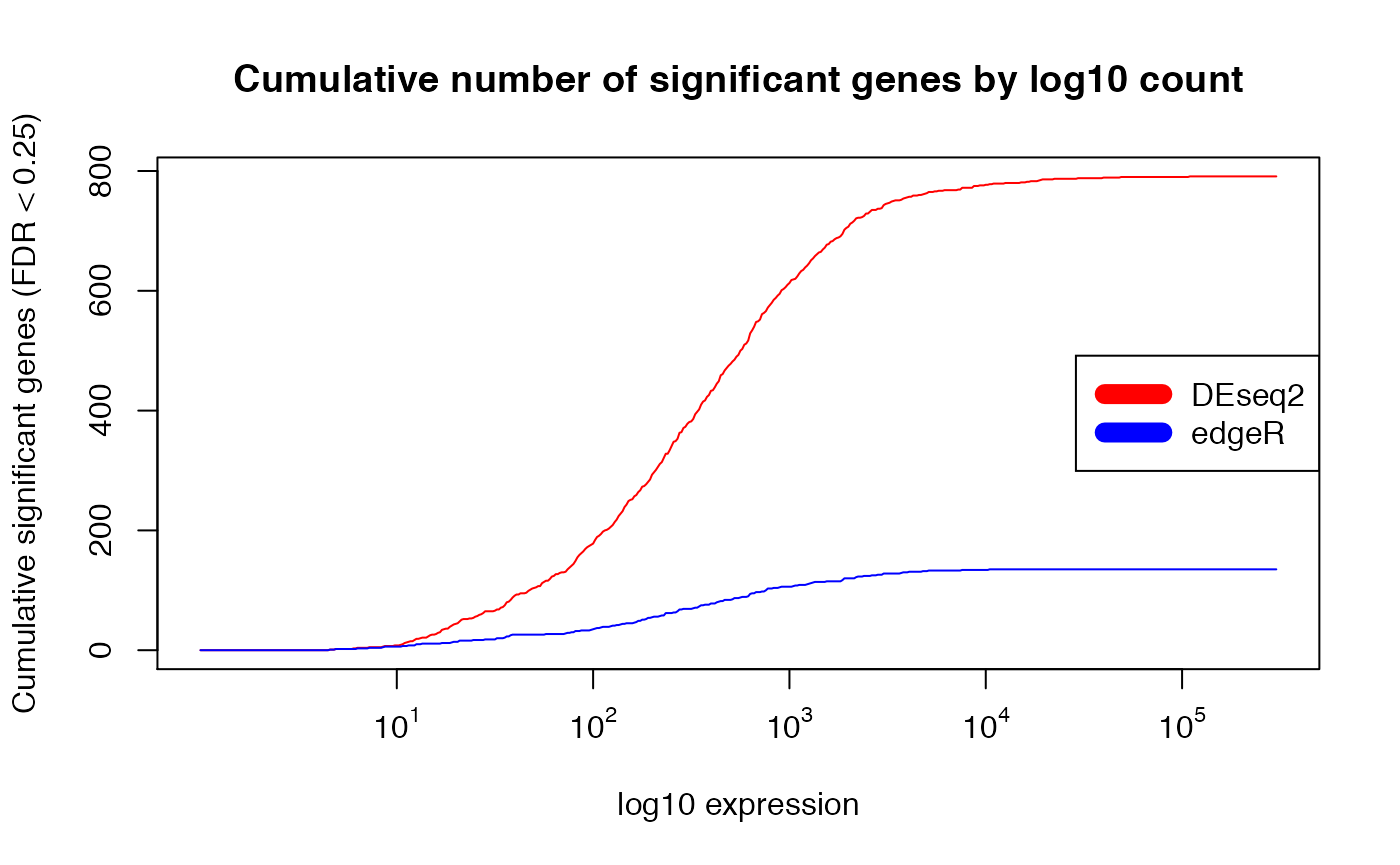
## normalization to proportion of significant genes instead of absolute number
##
plot(exprs_breaks, csg_DESeq2/max(csg_DESeq2),
     type = "l",
     col = "red",
     xaxt="n",
     xlab = "log10 expression",
     ylab = paste0("Cumulative proportion of significant genes (FDR < ", min.fdr, ")"),
     main = "Cumulative proportion of significant genes by log10 count")
lines(exprs_breaks, csg_edgeR/max(csg_edgeR), type = "l", col = "blue")
labels <- sapply(1:5,function(i) as.expression(bquote(10^ .(i))))
axis(1,at=1:5,labels=labels)
legend("right", c("DEseq2", "edgeR"), col=c("red", "blue", "yellow"), lwd=10)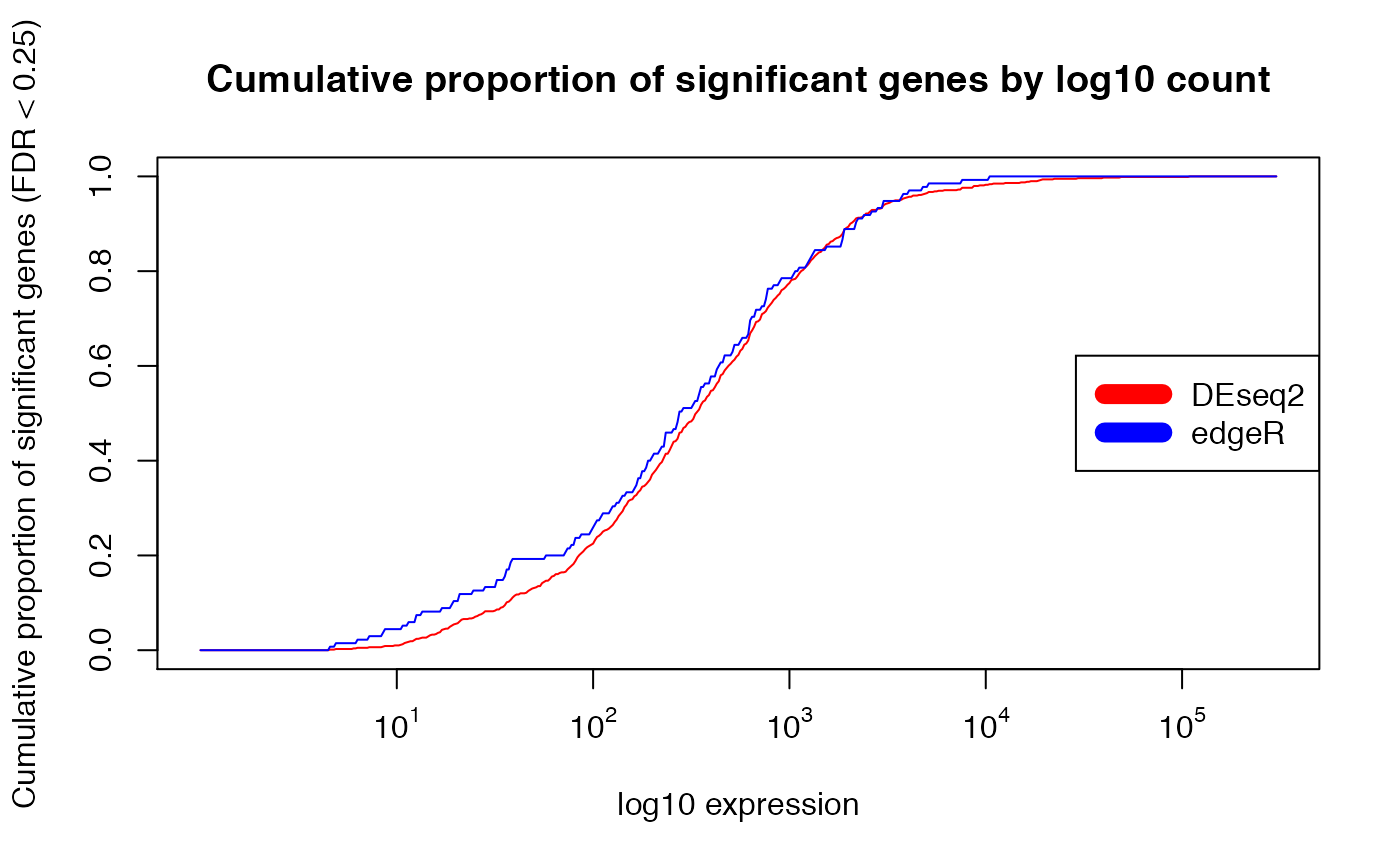
## histogram of proportion of sig genes by mean expression
##
hist(subset(res_summary, deseq2_padj < min.fdr)[, "mean_exprs"], freq=FALSE,
     col=rgb(1,0,0,1/4), xlab = "log10 expression",
     ylab = "number of sig. genes (fdr<0.25)",
     main = "Proportion of number of significant genes by log10 count", xaxt = "n")
hist(subset(res_summary, edgeR_padj < min.fdr)[, "mean_exprs"],freq=FALSE,
     col=rgb(0,0,1,1/4), add = T)
labels <- sapply( 1:5,function(i) as.expression(bquote(10^ .(i))) )
axis(1,at=1:5,labels=labels)
box()
legend("topright", c("DEseq2", "edgeR"),
  col=c(rgb(1,0,0,1/4), rgb(0,0,1,1/4), rgb(1,1,0,1/4)), lwd=10)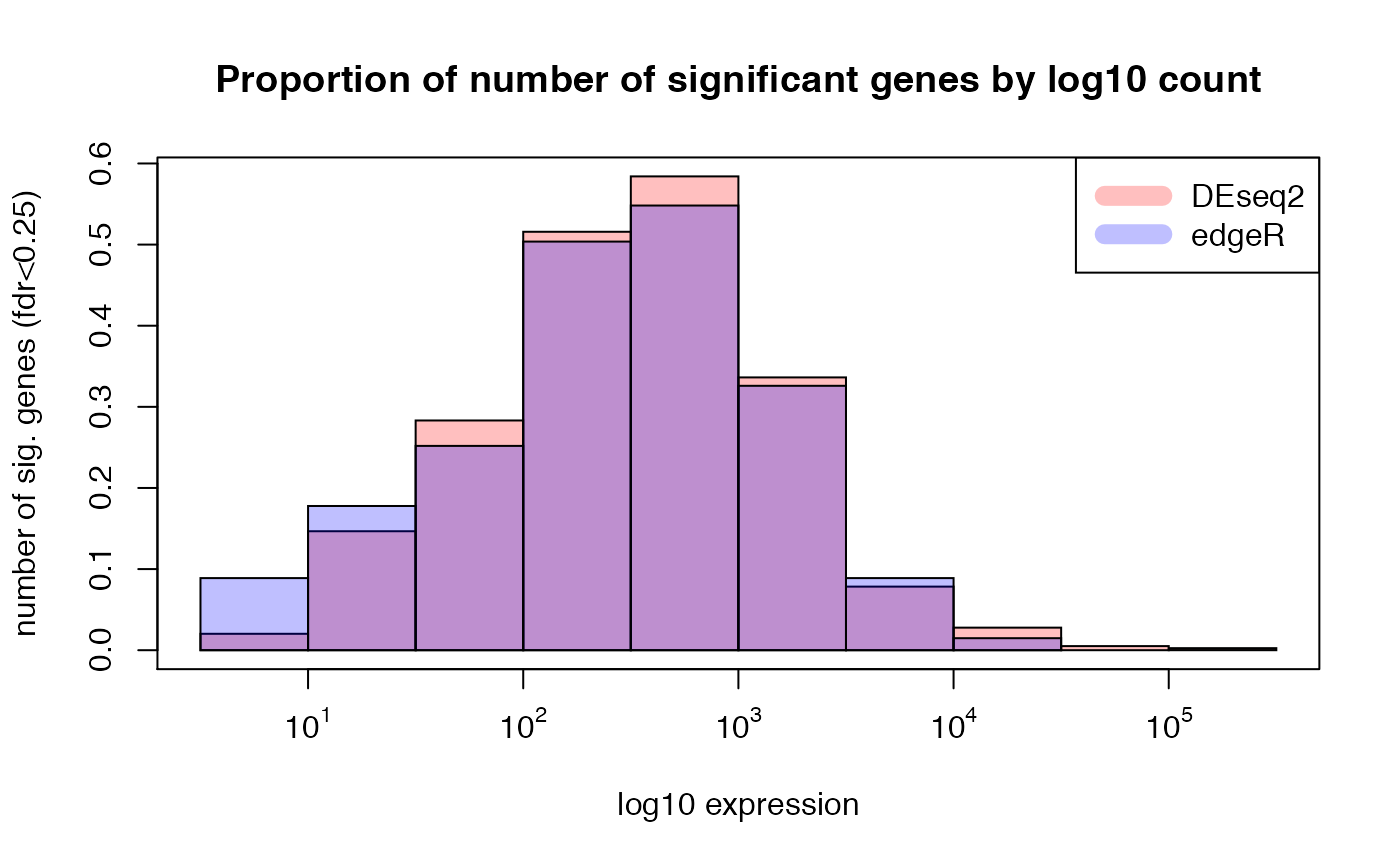
## expected results: DESeq claims edgeR is anti-conservative for lowly expressed genes, and
## more conservative for strongly expressed genes (weakly expressed genes overrepresented)
Comparison of DEseq vs. Limma(log2 data)
plot(exprs_breaks, csg_DESeq2,
     type = "l",
     col = "red",
     xaxt="n",
     xlab = "log10 expression",
     ylab = paste0("Cumulative significant genes (FDR < ", min.fdr, ")"),
     main = "Cumulative significant genes by log10 count")
lines(exprs_breaks, csg_limma, type = "l", col = "green")
labels <- sapply(1:5,function(i) as.expression(bquote(10^ .(i))))
axis(1,at=1:5,labels=labels)
legend("bottomright", c("DEseq2",  "limma"), col=c("red",  "green"), lwd=10)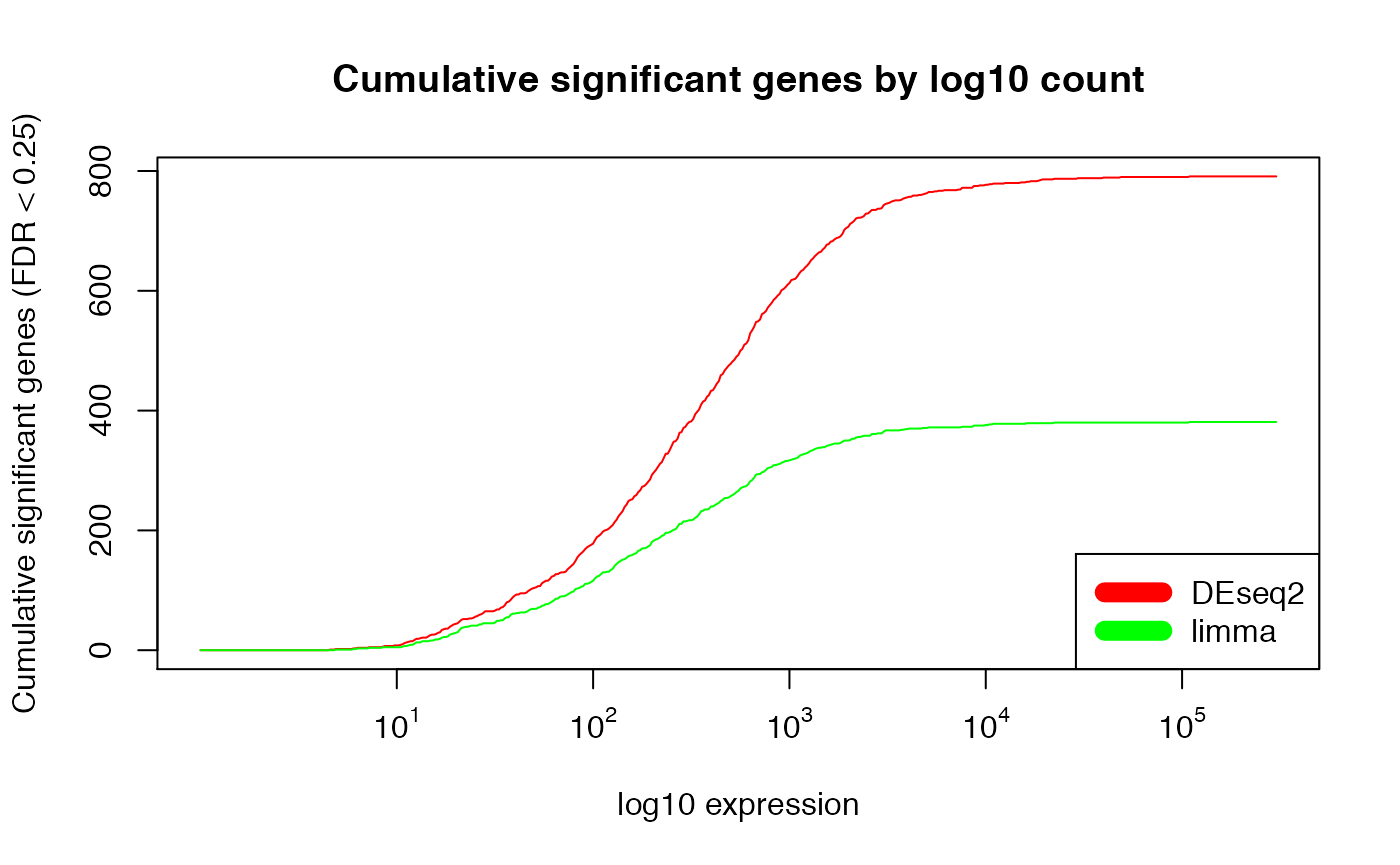
plot(exprs_breaks, csg_DESeq2/max(csg_DESeq2),
     type = "l",
     col = "red",
     xaxt="n",
     xlab = "log10 expression",
     ylab = paste0("Cumulative proportion of significant genes (fdr < ", min.fdr, ")"),
     main = "Cumulative proportion of significant genes by log10 count")
lines(exprs_breaks, csg_limma/max(csg_limma), type = "l", col = "green")
labels <- sapply(1:5,function(i) as.expression(bquote(10^ .(i))))
axis(1,at=1:5,labels=labels)
legend("right", c("DEseq2",  "limma"), col=c("red",  "green"), lwd=10)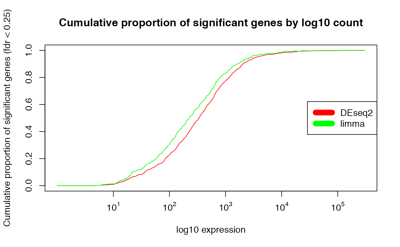
## histogram of proportion of sig genes by mean expression
hist(subset(res_summary, deseq2_padj < min.fdr)[, "mean_exprs"], freq=FALSE,
     col=rgb(1,0,0,1/4), xlab = "log10 expression",
     ylab = paste0("number of sig. genes (fdr < ", min.fdr, ")"),
     main = "Proportion of number of significant genes by log10 count", xaxt = "n")
hist(subset(res_summary, limma_padj < min.fdr)[, "mean_exprs"],freq=FALSE,
     col=rgb(1,1,0,1/4), add = T)
labels <- sapply( 1:5, function(i) as.expression(bquote(10^ .(i))) )
axis(1,at=1:5,labels=labels)
box()
legend("topright", c("DEseq2", "limma"), col=c(rgb(1,0,0,1/4),rgb(1,1,0,1/4)), lwd=10)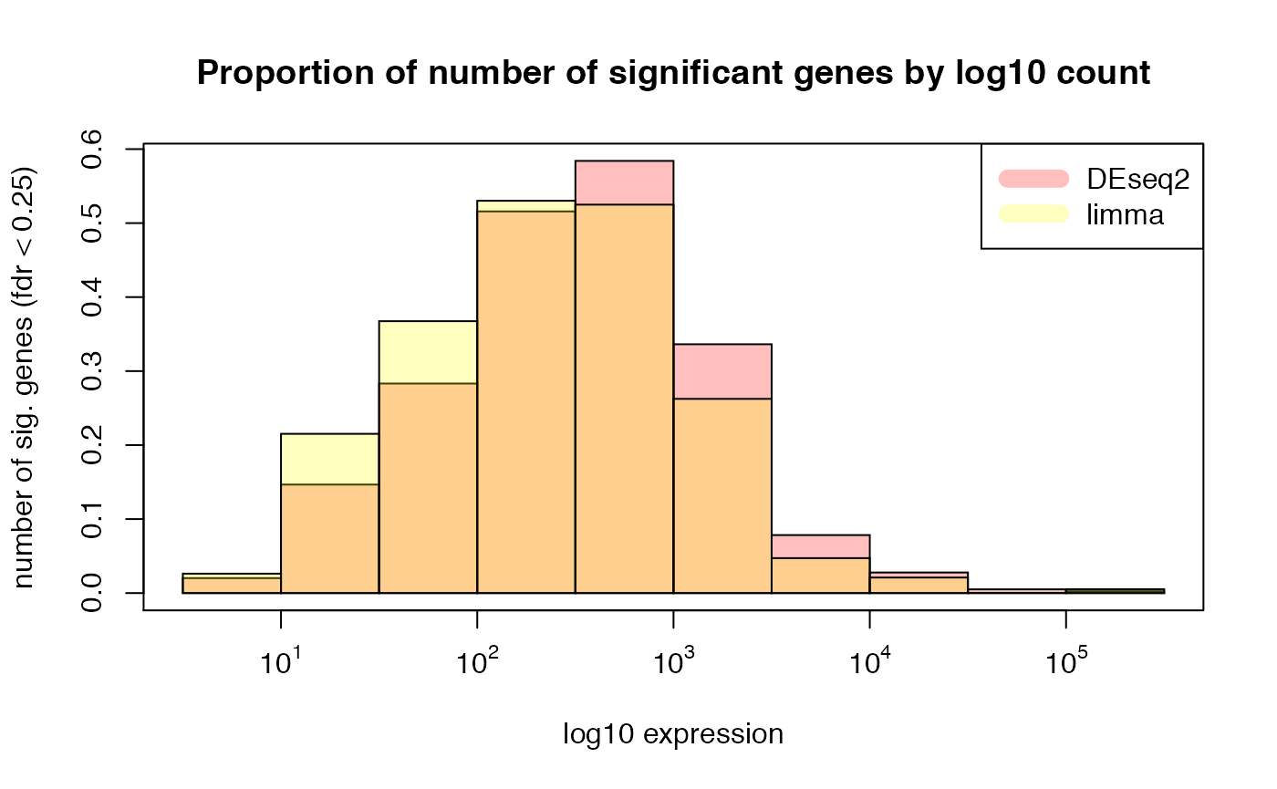
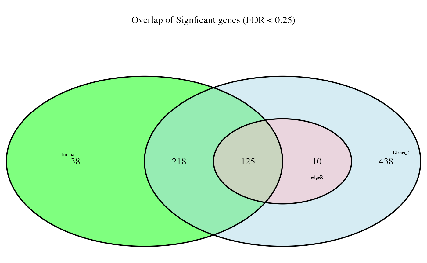
Venn Diagrams of Gene Signatures**
## looking at overlap of significant genes from the three tools
##
diff_list <- list(DESeq2 = rownames(subset(res_summary, deseq2_padj < min.fdr)),
  edgeR = rownames(subset(res_summary, edgeR_padj < min.fdr)),
  limma = rownames(subset(res_summary, limma_padj < min.fdr)))

fill <- c("light blue", "pink", "green")
size  <- rep(0.5, 3)
venn <- venn.diagram(x = diff_list,
                     filename = NULL,
                     height = 2000,
                     width = 2000, fill = fill,
                     cat.default.pos = "text",
                     cat.cex = size,
                     main = paste0("Overlap of Signficant genes (FDR < ", min.fdr, ")"))
grid.draw(venn)