Here we describe the definition and use of few simple functions to generate data and to plot from a univariate mixture of Normal distributions. According to R conventions, we define the four functions rmixnorm, pmixnorm, dmixnorm, and qmixnorm. These functions are defined in the file mixnorm.R. We also briefly introduce the package Mclust (see Quick Tour).
A simple mixnorm function
Below we define simple functions for sampling from, and computing the density of, Gaussian mixtures. In particular, inspect the function rmixnorm for the operational definition of the Data Generating Process discussed in class. We have also defined a function plot.mixnorm (in code/mixnorm.R, not shown here) for plotting a mixnorm’s density function. See Distributions.Rmd for more details on how to write a density plotting function.
## show the code
print(rmixnorm)
## function( size=1, p=c(1.0), mu=c(0.0), sigma=c(1.0) )
## {
## # generate from sum_j p_j N(mu_j,sigma_j)
## #
##
## # some checks on the input
## #
## if ( abs(sum(p)-1.0)>1.0e-5 ) { stop( "p's must sum to 1" ) }
## if ( length(p)!=length(mu) ) { stop( "length(p)!=length(mu)" ) }
## if ( length(p)!=length(sigma) ) { stop( "length(p)!=length(sigma)" ) }
##
## J <- length(p)
## if ( J==1 ) {
## return( rnorm(size,mu[1],sigma[1]) )
## }
## z <- sample(x=J,size=size,replace=TRUE,prob=p)
## n <- tabulate(z,nbins=J)
## y <- rep( NA, size )
## for ( j in (1:J) )
## {
## y[z==j] <- rnorm( n[j], mu[j], sigma[j] )
## }
## return( y )
## }
## <environment: namespace:BS831>
print(dmixnorm)## function( x, p=c(1.0), mu=c(0.0), sigma=c(1.0) )
## {
## matrix(sapply(x, dnorm, mean=mu, sd=sigma), length(x), length(p), byrow=T) %*% p
## }
## <environment: namespace:BS831>Below, we generate a sample from a 3-component Gaussian mixture, and show the data histogram together with the density plot.
set.seed(345) # for reproducible results
M3 <- rmixnorm(500,p=rep(1/3,3),mu=c(0,5,10),sigma=c(1,2,3))
hist(M3,probability=TRUE)
plot.mixnorm(1000,p=rep(1/3,3),mu=c(0,5,10),sigma=c(1,2,3),add=TRUE)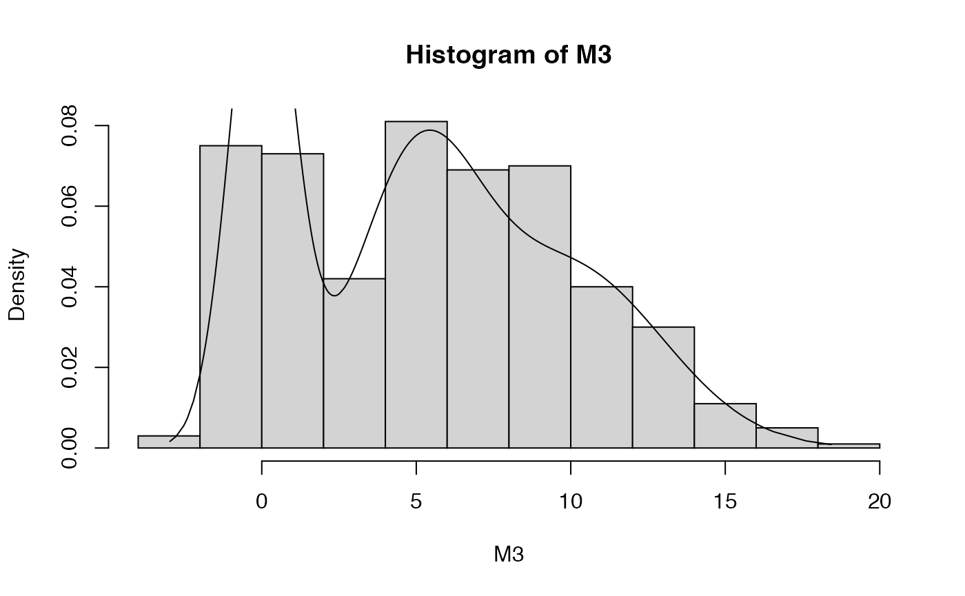
## Plot's truncated. Let's try the other way around ..
plot.mixnorm(1000,p=rep(1/3,3),mu=c(0,5,10),sigma=c(1,2,3))
hist(M3,probability=TRUE,add=TRUE)
abline(v=c(0,5,10),lty=3,col='red')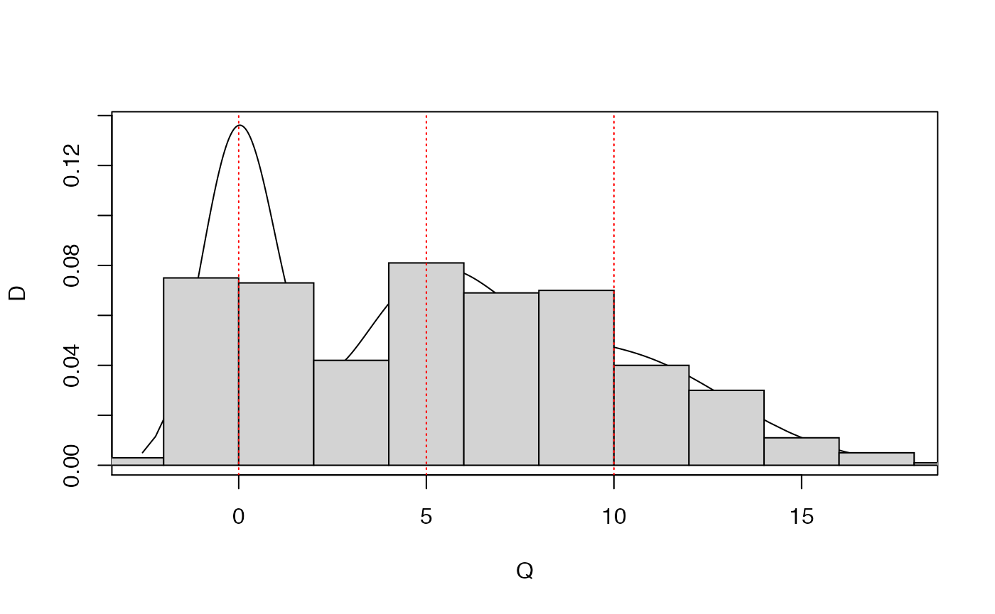
The MClust package
Here we briefly show the use of MClust (see vignette), a package that implements the fitting of Gaussian mixture models (univariate and multivariate), and which uses Expectation Maximization (EM) for parameter estimation, and the BIC approximation of the marginal likelihood P(D|M) for model selection. We start by fitting and testing models with between 1 and 6 mixture components with unequal (i.e., cluster-specific) variances.
## ----------------------------------------------------
## Gaussian finite mixture model fitted by EM algorithm
## ----------------------------------------------------
##
## Mclust V (univariate, unequal variance) model with 2 components:
##
##  log-likelihood   n df       BIC       ICL
##       -1420.269 500  5 -2871.612 -2947.839
##
## Clustering table:
##   1   2
## 144 356
print(MC3fit$parameters)## $pro
## [1] 0.2497157 0.7502843
##
## $mean
## 1 2
## -0.02596149 7.28405804
##
## $variance
## $variance$modelName
## [1] "V"
##
## $variance$d
## [1] 1
##
## $variance$G
## [1] 2
##
## $variance$sigmasq
## [1] 1.113905 14.396095
##
## $variance$scale
## [1] 1.113905 14.396095
## boxplot the data as a function of their cluster assignment
boxplot(M3~MC3fit$classification)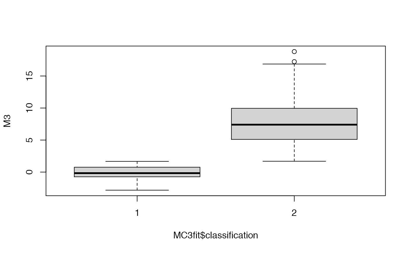
Even with 500 points, because of the large variance of the 2nd and 3rd components, the fitting procedure was not capable of guessing the ‘correct’ number of clusters. Let’s try by either increasing the sample size or decreasing the variance.
set.seed(123)
## increase the sample size
M3 <- rmixnorm(5000,p=rep(1/3,3),mu=c(0,5,10),sigma=c(1,2,3))
plot.mixnorm(5000,p=rep(1/3,3),mu=c(0,5,10),sigma=c(1,2,3),main="5,000 data points")
hist(M3,probability=TRUE,add=TRUE)
abline(v=c(0,5,10),lty=3,col='red')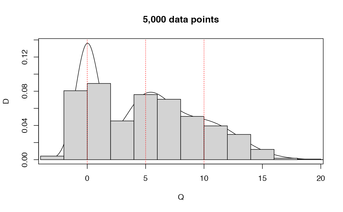
## ----------------------------------------------------
## Gaussian finite mixture model fitted by EM algorithm
## ----------------------------------------------------
##
## Mclust V (univariate, unequal variance) model with 3 components:
##
##  log-likelihood    n df       BIC      ICL
##       -13959.68 5000  8 -27987.51 -29428.3
##
## Clustering table:
##    1    2    3
## 1751 1766 1483
print(MC3fit$parameters)## $pro
## [1] 0.3394103 0.3340429 0.3265468
##
## $mean
## 1 2 3
## 0.02159402 5.10997555 10.09963049
##
## $variance
## $variance$modelName
## [1] "V"
##
## $variance$d
## [1] 1
##
## $variance$G
## [1] 3
##
## $variance$sigmasq
## [1] 1.036242 3.580035 8.569311
##
## $variance$scale
## [1] 1.036242 3.580035 8.569311
## boxplot the data as a function of their cluster assignment
boxplot(M3~MC3fit$classification)
abline(h=MC3fit$parameters$mean,col="red",lty=3)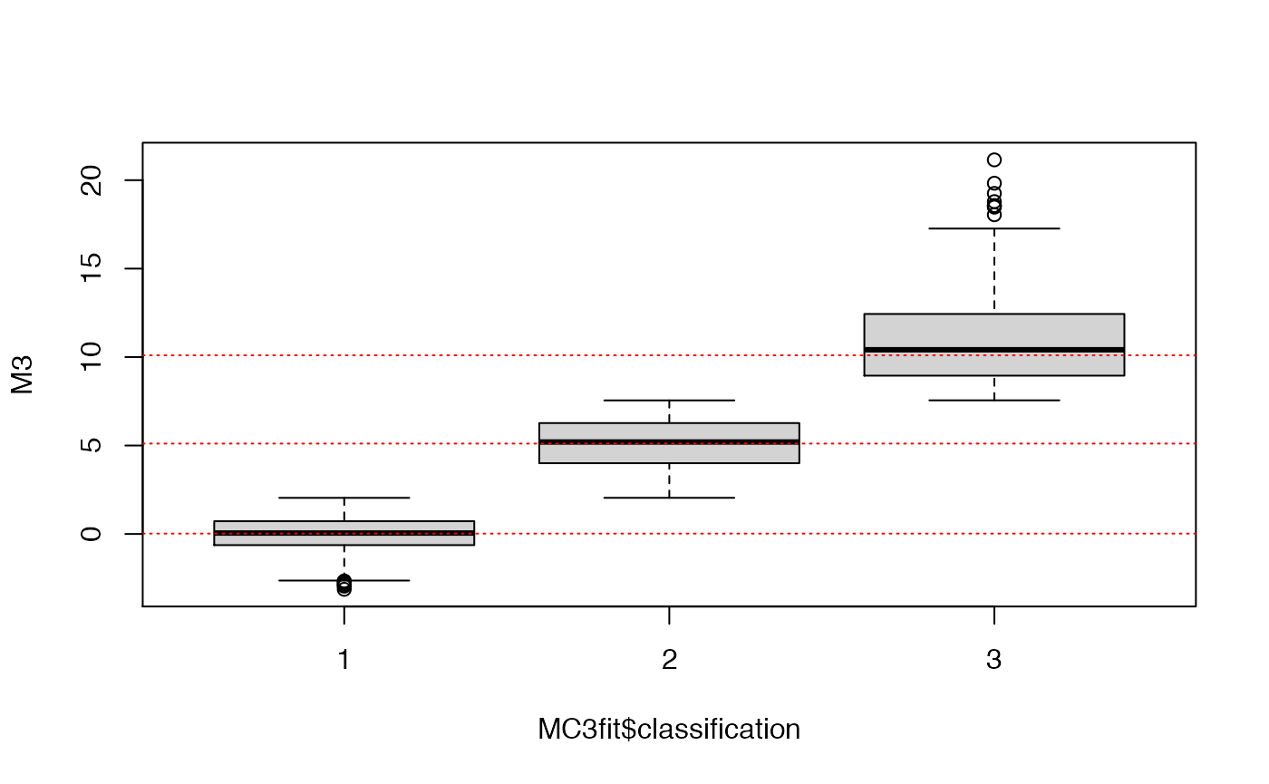
## decrease the variance
set.seed(123)
M3 <- rmixnorm(500,p=rep(1/3,3),mu=c(0,5,10),sigma=c(1,1,1))
plot.mixnorm(500,p=rep(1/3,3),mu=c(0,5,10),sigma=c(1,1,1),main="500 data points")
hist(M3,probability=TRUE,add=TRUE)
abline(v=c(0,5,10),lty=3,col='red')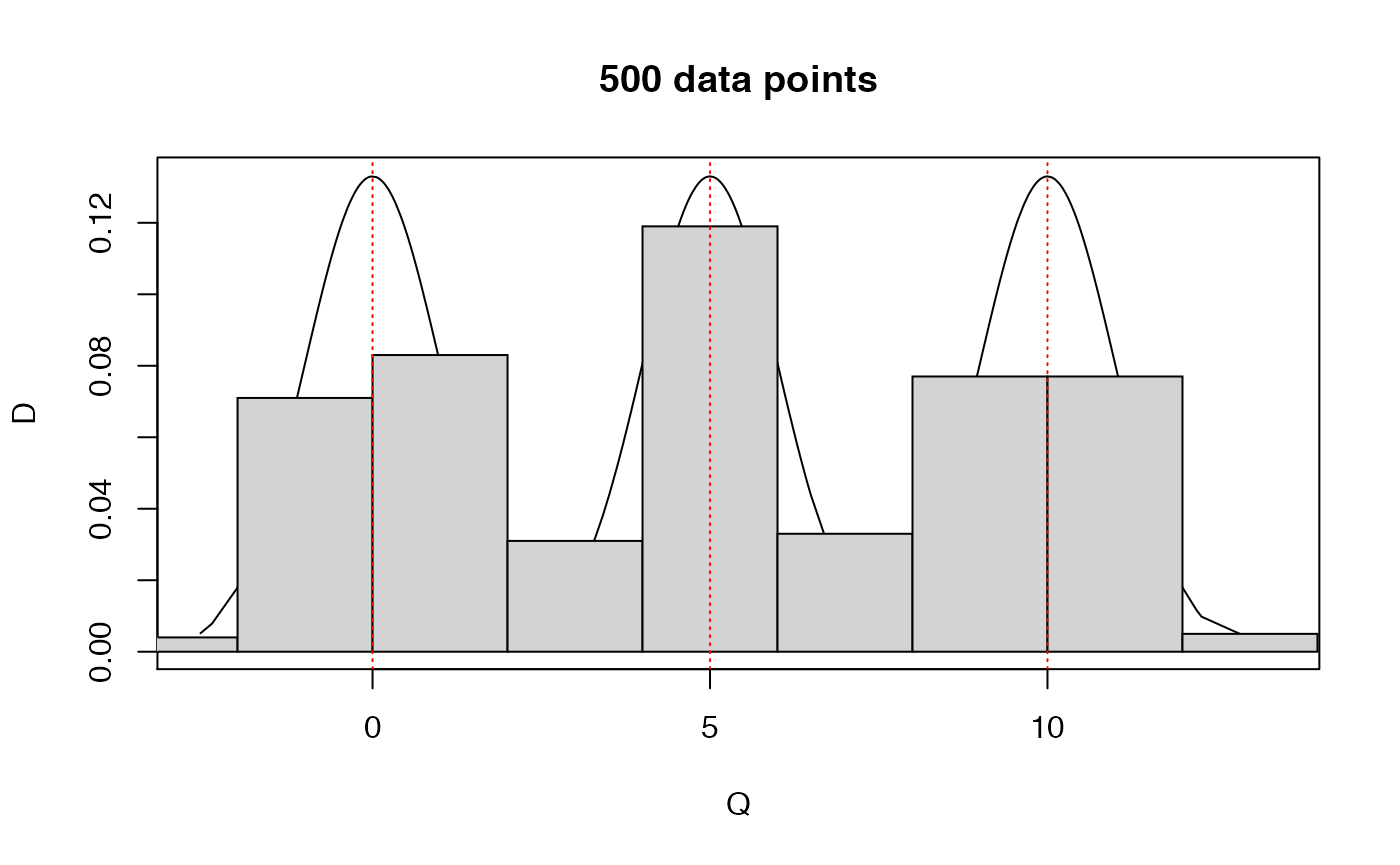
## ----------------------------------------------------
## Gaussian finite mixture model fitted by EM algorithm
## ----------------------------------------------------
##
## Mclust V (univariate, unequal variance) model with 3 components:
##
##  log-likelihood   n df       BIC       ICL
##       -1249.092 500  8 -2547.901 -2559.198
##
## Clustering table:
##   1   2   3
## 165 170 165
print(MC3fit$parameters)## $pro
## [1] 0.3298465 0.3423652 0.3277883
##
## $mean
## 1 2 3
## 0.07608453 5.09150649 9.95602964
##
## $variance
## $variance$modelName
## [1] "V"
##
## $variance$d
## [1] 1
##
## $variance$G
## [1] 3
##
## $variance$sigmasq
## [1] 1.0499845 0.8611873 1.1545231
##
## $variance$scale
## [1] 1.0499845 0.8611873 1.1545231