Differential Analysis as Linear Regression

This is the code for the plot shown in slide #48 of BS831_class03_ComparativeExperimentLM.Rmd (“Differential Analysis as linear regression (LM)”).

set.seed(159) # for reproducible results 
nobs <- 10000 # sample size
beta0 <- 5    # mean in class 0
beta1 <- 1.5  # beta0 + this is mean in class 1
X <- sample(0:1,nobs,replace=TRUE)
Y <- rnorm(nobs,mean=beta0 + beta1 * X,sd=1)

## or, equivalently
## Y <- beta0 + beta1 * X + rnorm(nobs,mean=0,sd=1)

par(mar=c(c(5, 4, 4, 5) + 0.1))
boxplot(Y~X,ylab="Y",pch="-",names=paste("X =",0:1),col="antiquewhite")
abline(h=c(beta0=beta0,'beta0+beta1'=beta0+beta1),col="red",lty=3,lwd=2)

## notice the use of 'expression' to display mathematical symbols
axis(side=4,at=c(beta0,beta0+beta1),labels=expression(beta[0],beta[0]+beta[1]),las=1)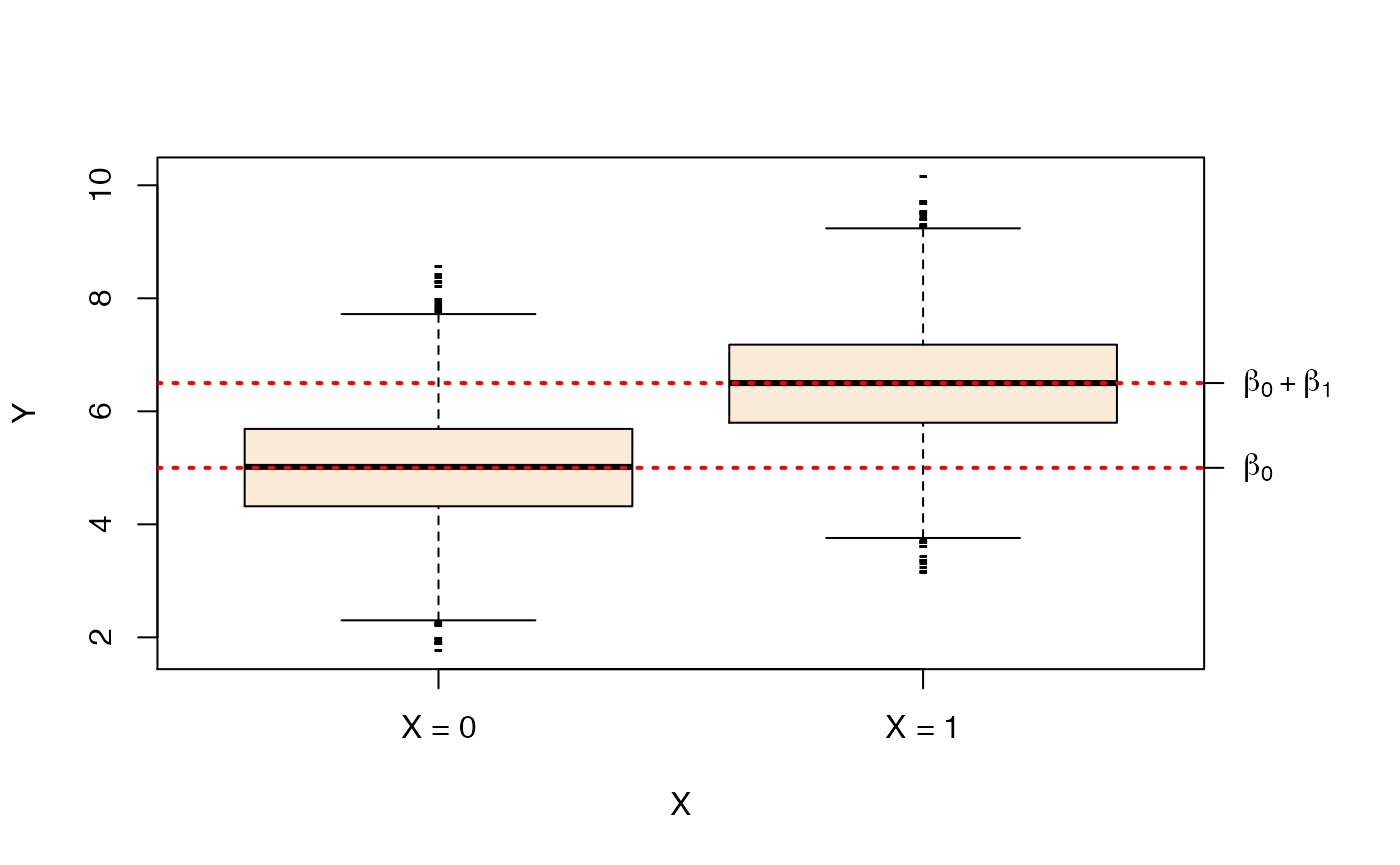

We now fit a linear model to the generated data by lm.

LM <- lm(Y ~ X)
print(summary(LM))

## 
## Call:
## lm(formula = Y ~ X)
## 
## Residuals:
##     Min      1Q  Median      3Q     Max 
## -3.3417 -0.6872  0.0121  0.6879  3.6653 
## 
## Coefficients:
##             Estimate Std. Error t value Pr(>|t|)    
## (Intercept)  4.99939    0.01435  348.29   <2e-16 ***
## X            1.49248    0.02026   73.68   <2e-16 ***
## ---
## Signif. codes:  0 '***' 0.001 '**' 0.01 '*' 0.05 '.' 0.1 ' ' 1
## 
## Residual standard error: 1.013 on 9998 degrees of freedom
## Multiple R-squared:  0.3519, Adjusted R-squared:  0.3519 
## F-statistic:  5429 on 1 and 9998 DF,  p-value: < 2.2e-16

As you can see, the estimates are quite close to the generating parameters.

Stefano Monti