Multiple-Hypothesis Correction
Stefano Monti
Source:vignettes/docs/MHTcorrection.Rmd
MHTcorrection.RmdIn this module, we show how testing for multiple hypotheses (genes) can increase the chance of false positives, especially for small sample sizes.
Multiple-Hypothesis Correction by FDR and FWER
In the remainder of this module we will explore the effects of multiple hypothesis corrections on family-wise error rate, false positive rate, false negative rate, and power when using Bonferroni and Benjamini Hochberg corrections.
Define functions
The following function is just a wrapper for runnning two-sample t-tests.
Wrapper of Student’s T-Test
## wrapper function extracting t-statistic and p-value from a call to function t.test
tscore <- function(y,x) {
  tmp <- t.test(y~x)
  c(score=tmp$statistic,pval=tmp$p.value)
}
The next function is a wrapper to define a data matrix, X, and outcome vector, Y, for different conditions. By default we can generate a complete set of data from the null hypthesis to check the FWER. We can also generate data with a subset of features which have different means between groups to check, false positive rate, false negative rate, and power by changing propDiff and Diff.
Wrapper of data generation and differential analysis
wrapDA <- function(Nsamps, # Number of samples per pseudogroup
                   Nrow = 200, # Number of parameters
                   mean = 0, # Mean of normal
                   sd = 0.5, # SD of normal
                   alpha = 0.05, # Signficance threshold
                   propDiff = 0, # Proportion to make Ha
                   Diff = 0, # Difference for Ha features
                   reportAll = FALSE
                   )
  {

  # Genreate a data of random data from null distribution
  DAT <- matrix( rnorm( Nrow * Nsamps * 2, mean=0, sd=0.5), nrow=Nrow, ncol=( Nsamps *2) )

  # Add difference to one group
  if(propDiff > 0){
    nChange <- floor(propDiff*Nrow)
    DAT[1:(nChange), 1:Nsamps] <- DAT[1:(nChange), 1:Nsamps] + Diff
    rownames(DAT) <- paste0(c(rep("Ha", nChange), rep("H0", (Nrow - nChange))), 1:Nrow)
  }

  ## generate a (head/tail) phenotype of proper size
  pheno <- factor(rep(c('head','tail'),each=Nsamps))

  ## perform t.test on each data row with respect to the random phenotype
  DIF <- as.data.frame(t(apply(DAT,1,tscore,x=pheno)))

  ## Sort by p-value
  DIF <- DIF[order(DIF$pval),]

  ## Perform Bonferroni and BH corrections
  DIF$BFp <- p.adjust(DIF$pval, method = "bonferroni")
  DIF$BHp <- p.adjust(DIF$pval, method = "BH")

  ## Get BH Significant Rows
  DIFsig <- DIF[DIF$BHp < alpha,]

  ## Return All results or only features with small p-values
  if(reportAll){
    return(DIF)
  } else {
    ## If any genes BH significant return these rows else just return row with smallest p-value
    if(nrow(DIFsig)>0) return(DIFsig) else return(DIF[1,])
  }
}
Run differential analysis from null distributions for different sample sizes
First, we will check the FWER between Bonferroni and BH corrections for two different sample sizes: 10 samples per group and 50 samples per group. Each feature will have mean=0 and SD=0.5. For each run, the result will either be the feature with the smallest p-value, or a data.frame of features that passed BH significance threshold.
sGroups <- c(10, 25, 50) # Vector of group sizes

# Run simulation for each sample size 100 times
outList <- lapply(sGroups, function(Nsamps){
    replicate(100, wrapDA(Nsamps), simplify = FALSE)
})

# Name list by sample size
names(outList) <- paste("Samps", sGroups, sep = "_")

# What does the output look like?
outList$Samps_10[[1]]
## score.t pval BFp BHp
## 51 3.331967 0.003733701 0.7467403 0.4291216Get family wise error rates from Bonferroni (alpha = 0.05)
Function to calculate FWER from list of experiment results
getFWER <- function(resList, # List of lowest p-values
                    alpha = 0.05, # P-value threshold
                    pCol = "BFp" # Column with MHT P-value of interest
                    )
{
  ## Which experiments had at least one positive hit?
  FWERvec <- unlist(lapply(resList, function(y) sum(y[,"BFp"] < alpha)>0))

  ## What proportion of experiments had at least one positive hit?
  FWERval <- mean(FWERvec)

  ## Return FWER for this set of experiments
  return(FWERval)
}
## Get FWER for bonferonni corrected p-values
BonVec <- unlist(lapply(outList, getFWER, alpha = 0.05, pCol = "BFp")) # Note pCol
print(BonVec)
## Samps_10 Samps_25 Samps_50
## 0.03 0.05 0.06
## Get FWER for Benjamini-Hochberg corrected p-values
BhVec <- unlist(lapply(outList, getFWER, alpha = 0.05, pCol = "BHp")) # Note pCol
print(BhVec)
## Samps_10 Samps_25 Samps_50
## 0.03 0.05 0.06Note, for repeated experiments with multiple hypotheses the FWER returned from Bonferroni and Benjamini-Hochberg is the same
Run differential analysis from alternative distriubtions for different sample sizes
Next, we will create data where 25% of the genes differ between groups by 0.5. In the output, true positive will have row names starting with “Ha”.
haList <- lapply(sGroups, function(Nsamps){
    replicate(100, wrapDA(Nsamps, propDiff = 0.25, Diff = 0.5), simplify = FALSE)
})

## Name list by sample size
names(haList) <- paste("Samps", sGroups, sep = "_")

## What does the output look like?
haList$Samps_10[[1]]
## score.t pval BFp BHp
## Ha25 5.890020 2.423153e-05 0.004846306 0.004846306
## Ha11 5.141227 7.018181e-05 0.014036362 0.007018181
## Ha46 4.824875 1.422735e-04 0.028454700 0.009484900
## Ha22 4.690544 2.178593e-04 0.043571869 0.010892967The rows with the prefix, Ha, come from the distribution for which the alternative hypthesis is true.
Get False Positive and False Negative Rates
Function to calculate the false positive rate and false negative rates from list of experiment results
The a false positive rate will be calculated for each experiment individually
getFPR_FNR <- function(resList, # List of lowest p-values
                       alpha = 0.05, # P-value threshold
                       pCol = "BFp", # Column with MHT P-value of interest
                       nMH = 200, # Number of hypothesis tested
                       nHa = 50 # Number of true positives
                       )
{
  ## Extract instances of null hypotheses with small p-values from each experiment
  H0list <- lapply(resList, function(y) y[!grepl("Ha", rownames(y)),])

  # Extract vector of false postive rates from each experiment
  FPvec <- unlist(lapply(H0list, function(y) sum(y[,pCol]<alpha)/(nMH-nHa)))

  # Extract instances of alternative hypotheses with small p-values from each experiment
  Halist <- lapply(resList, function(y) y[grepl("Ha", rownames(y)),])

  # Extract vector of false negative rates from each experiment
  FNvec <- 1 - unlist(lapply(Halist, function(y) sum(y[,pCol]<alpha)/(nHa)))

  # Create data.frame of results
  FP_FN <- data.frame(FalsePosi = FPvec, FalseNeg = FNvec)

  return(FP_FN)
}
Bonferroni Corrected P-values
## Get FP and FN
BonFP_FN <- lapply(haList, getFPR_FNR, alpha = 0.05, pCol = "BFp", nMH = 200, nHa = 50)

## Concatenate the results for each sample size
BonFP_FN <- do.call(rbind, BonFP_FN)
head(BonFP_FN)
## FalsePosi FalseNeg
## Samps_10.1 0 0.92
## Samps_10.2 0 0.96
## Samps_10.3 0 1.00
## Samps_10.4 0 1.00
## Samps_10.5 0 0.98
## Samps_10.6 0 1.00
## Add column for sample size identifier
BonFP_FN$SampleSize <- sub("[.][[:digit:]]*", "", rownames(BonFP_FN))
head(BonFP_FN)
## FalsePosi FalseNeg SampleSize
## Samps_10.1 0 0.92 Samps_10
## Samps_10.2 0 0.96 Samps_10
## Samps_10.3 0 1.00 Samps_10
## Samps_10.4 0 1.00 Samps_10
## Samps_10.5 0 0.98 Samps_10
## Samps_10.6 0 1.00 Samps_10Benjamini Hochberg Corrected P-values
## Get FP and FN
BhFP_FN <- lapply(haList, getFPR_FNR, alpha = 0.05, pCol = "BHp", nMH = 200, nHa = 50)

## Concatenate the results for each sample size
BhFP_FN <- do.call(rbind, BhFP_FN)
head(BhFP_FN)
## FalsePosi FalseNeg
## Samps_10.1 0.000000000 0.92
## Samps_10.2 0.006666667 0.86
## Samps_10.3 0.000000000 1.00
## Samps_10.4 0.000000000 0.86
## Samps_10.5 0.000000000 0.90
## Samps_10.6 0.000000000 1.00
## Add column for sample size identifier
BhFP_FN$SampleSize <- sub("[.][[:digit:]]*", "", rownames(BhFP_FN))
head(BhFP_FN)
## FalsePosi FalseNeg SampleSize
## Samps_10.1 0.000000000 0.92 Samps_10
## Samps_10.2 0.006666667 0.86 Samps_10
## Samps_10.3 0.000000000 1.00 Samps_10
## Samps_10.4 0.000000000 0.86 Samps_10
## Samps_10.5 0.000000000 0.90 Samps_10
## Samps_10.6 0.000000000 1.00 Samps_10Plot Results
We will create boxplots of the results with ggplot2.
## Concatenate results between Bonferroni and Benjamini-Hochberg
FP_FN <- rbind(BonFP_FN, BhFP_FN)
FP_FN$correction <- rep(c("Bonferroni", "BH"), each = nrow(BonFP_FN)) # Add correction type
head(FP_FN)
## FalsePosi FalseNeg SampleSize correction
## Samps_10.1 0 0.92 Samps_10 Bonferroni
## Samps_10.2 0 0.96 Samps_10 Bonferroni
## Samps_10.3 0 1.00 Samps_10 Bonferroni
## Samps_10.4 0 1.00 Samps_10 Bonferroni
## Samps_10.5 0 0.98 Samps_10 Bonferroni
## Samps_10.6 0 1.00 Samps_10 Bonferroni
## Create one column of False Positive and False Negative Rates
FP_FN <- gather(FP_FN, key = "statistic", value = "measure", 1:2)
head(FP_FN)
## SampleSize correction statistic measure
## 1 Samps_10 Bonferroni FalsePosi 0
## 2 Samps_10 Bonferroni FalsePosi 0
## 3 Samps_10 Bonferroni FalsePosi 0
## 4 Samps_10 Bonferroni FalsePosi 0
## 5 Samps_10 Bonferroni FalsePosi 0
## 6 Samps_10 Bonferroni FalsePosi 0
# Create plot of results
ggplot(FP_FN, aes(x = SampleSize,
                        y = measure,
                        fill = correction,
                        colour = correction)) +
  geom_boxplot() +
  facet_wrap(~statistic, nrow = 2, scales = "free_y")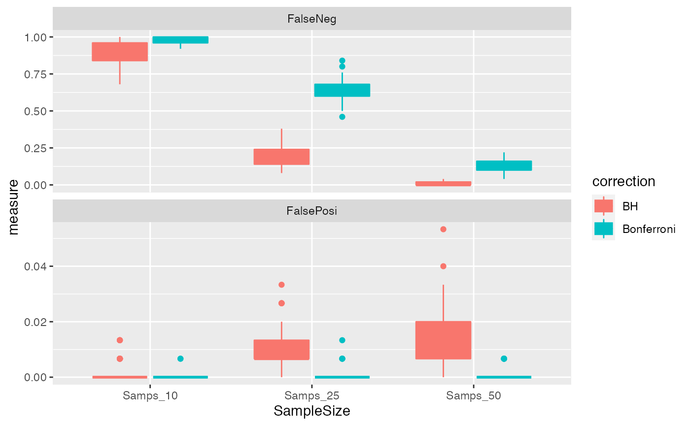
What do you notice about the nature of the performance of the FWER-based Bonferroni correction, and FDR-based Benjamini-Hochberg correction.