Relational Genesets
When dealing with hundreds of genesets, it’s often useful to understand the relationships between them. This allows researchers to summarize many enriched pathways as more general biological processes. To do this, we rely on curated relationships defined between them. For example, Reactome conveniently defines their genesets in a hiearchy of pathways. This data can be formatted into a relational genesets object called rgsets.
genesets <- hyperdb_rgsets("REACTOME", version="70.0")Relational genesets have three data atrributes including gsets, nodes, and edges. The genesets attribute includes the geneset information for the leaf nodes of the hiearchy, the nodes attribute describes all nodes in the hierarchy, including internal nodes, and the edges attribute describes the edges in the hiearchy.
print(genesets)REACTOME v70.0
Genesets
2-LTR circle formation (13)
5-Phosphoribose 1-diphosphate biosynthesis (3)
A tetrasaccharide linker sequence is required for GAG synthesis (26)
ABC transporters in lipid homeostasis (18)
ABO blood group biosynthesis (3)
ADP signalling through P2Y purinoceptor 1 (25)
Nodes
label
R-HSA-164843 2-LTR circle formation
R-HSA-73843 5-Phosphoribose 1-diphosphate biosynthesis
R-HSA-1971475 A tetrasaccharide linker sequence is required for GAG synthesis
R-HSA-5619084 ABC transporter disorders
R-HSA-1369062 ABC transporters in lipid homeostasis
R-HSA-382556 ABC-family proteins mediated transport
id length
R-HSA-164843 R-HSA-164843 13
R-HSA-73843 R-HSA-73843 3
R-HSA-1971475 R-HSA-1971475 26
R-HSA-5619084 R-HSA-5619084 77
R-HSA-1369062 R-HSA-1369062 18
R-HSA-382556 R-HSA-382556 22
Edges
from to
1 R-HSA-109581 R-HSA-109606
2 R-HSA-109581 R-HSA-169911
3 R-HSA-109581 R-HSA-5357769
4 R-HSA-109581 R-HSA-75153
5 R-HSA-109582 R-HSA-140877
6 R-HSA-109582 R-HSA-202733Passing relational genesets works natively with hypeR().
data(limma)

signature <- limma %>%
             dplyr::arrange(desc(t)) %>%
             magrittr::use_series(symbol)

hyp_obj <- hypeR(signature, genesets, test="kstest", fdr=0.01)
Interactive Visualization
One can visualize the top enriched genesets using hyp_hmap() which will return a hierarchy map. Each node represents a geneset, where the shade of the gold border indicates the normalized significance of enrichment. Hover over the leaf nodes to view the raw value. Double click internal nodes to cluster their first degree connections. Edges represent a directed relationship between genesets in the hiearchy. Note: This function only works when the hyp object was initialized with an rgsets object.
vn <- hyp_hmap(hyp_obj, top=30)
vn
Save to an html file.
Static Visualization
One of the downsides of the above interactive object is it’s difficult to render high quality figures in specific formats. You could take a screenshot after interacting with the figure, however that might not be high enough resolution for a publication. To help with this, you can alternatively return an igraph object pre-formatted with enrichment data.
IGRAPH aa0593f DN-B 92 83 --
+ attr: name (v/c), fdr (v/n), size (v/n), color (v/c), frame.color
| (v/c), label (v/c), type (v/c), label.family (v/c), label.color
| (v/c), label.font (v/n), label.cex (v/n), label.dist (v/n), width
| (e/n), color (e/c), arrow.size (e/n)
+ edges from aa0593f (vertex names):
 [1] R-HSA-109581 ->R-HSA-169911  R-HSA-1234174->R-HSA-1234176
 [3] R-HSA-1280215->R-HSA-5668541 R-HSA-1280215->R-HSA-9607240
 [5] R-HSA-1430728->R-HSA-71291   R-HSA-157118 ->R-HSA-9013694
 [7] R-HSA-162582 ->R-HSA-157118  R-HSA-162582 ->R-HSA-194315
 [9] R-HSA-162582 ->R-HSA-195721  R-HSA-162582 ->R-HSA-5358351
+ ... omitted several edges
Colors, weights, and normalized sizing properties from the interactive visualization are copied over to the vertex properties of the igraph object.
head(igraph::as_data_frame(ig, what="vertices"))[,c("name", "type", "fdr", "size", "color")] name type fdr size color
R-HSA-174178 R-HSA-174178 leaf 1.7e-05 15.00000 #C70039
R-HSA-174143 R-HSA-174143 internal NA 15.00000 #581845
R-HSA-453276 R-HSA-453276 internal NA 15.00000 #581845
R-HSA-69278 R-HSA-69278 internal NA 28.49315 #581845
R-HSA-1640170 R-HSA-1640170 internal NA 29.17808 #581845
R-HSA-450408 R-HSA-450408 leaf 1.0e-05 15.00000 #C70039Because genesets labels are typically long, it’s static visualizations are difficult. You’ll need to make custom adjustments depending on your needs.
# Consistent layout
set.seed(1)

# Overriding existing edge/vertex properties
plot(ig,
     vertex.label=substr(ifelse(V(ig)$type == "leaf", V(ig)$label, ""), 1, 32),
     vertex.size=5)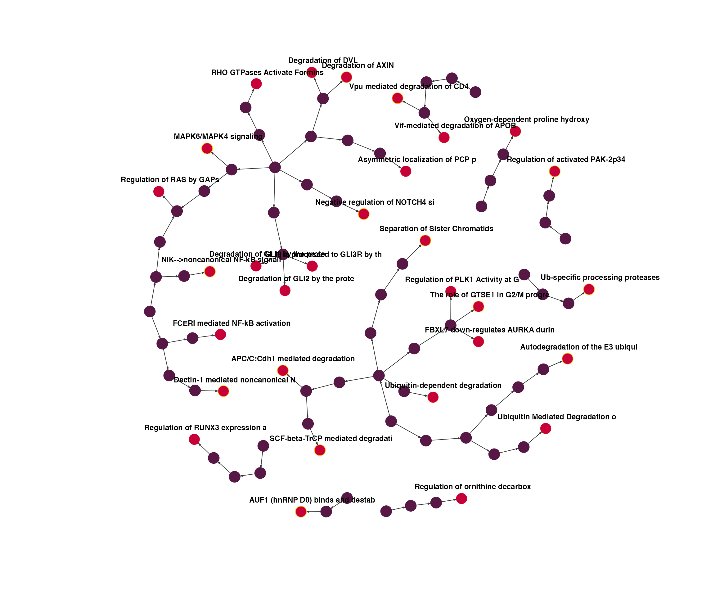
Raw Graph Objects
You can also directly copy enrichment data from a hyp object to an igraph object.
ig <- hyp_to_graph(hyp_obj)
print(ig)
IGRAPH c6922c7 DN-- 2255 2264 --
+ attr: name (v/c), label (v/c), pval (v/n), fdr (v/n), signature
| (v/n), geneset (v/n), overlap (v/n), score (v/n)
+ edges from c6922c7 (vertex names):
[1] R-HSA-109581->R-HSA-109606 R-HSA-109581->R-HSA-169911
[3] R-HSA-109581->R-HSA-5357769 R-HSA-109581->R-HSA-75153
[5] R-HSA-109582->R-HSA-140877 R-HSA-109582->R-HSA-202733
[7] R-HSA-109582->R-HSA-418346 R-HSA-109582->R-HSA-75205
[9] R-HSA-109582->R-HSA-75892 R-HSA-109582->R-HSA-76002
[11] R-HSA-109582->R-HSA-983231 R-HSA-109606->R-HSA-111452
[13] R-HSA-109606->R-HSA-111453 R-HSA-109606->R-HSA-111471
+ ... omitted several edges
df.v <- ig %>%
        igraph::as_data_frame(what="vertices") %>%
        dplyr::arrange(fdr)

head(df.v)
name
R-HSA-5687128 R-HSA-5687128
R-HSA-174113 R-HSA-174113
R-HSA-2467813 R-HSA-2467813
R-HSA-450408 R-HSA-450408
R-HSA-5676590 R-HSA-5676590
R-HSA-8852276 R-HSA-8852276
label pval
R-HSA-5687128 MAPK6/MAPK4 signaling 6.8e-11
R-HSA-174113 SCF-beta-TrCP mediated degradation of Emi1 1.6e-08
R-HSA-2467813 Separation of Sister Chromatids 1.3e-08
R-HSA-450408 AUF1 (hnRNP D0) binds and destabilizes mRNA 4.6e-08
R-HSA-5676590 NIK-->noncanonical NF-kB signaling 3.8e-08
R-HSA-8852276 The role of GTSE1 in G2/M progression after G2 checkpoint 4.1e-08
fdr signature geneset overlap score
R-HSA-5687128 1.1e-07 9682 94 62 0.44
R-HSA-174113 8.4e-06 9682 55 35 0.51
R-HSA-2467813 8.4e-06 9682 171 112 0.29
R-HSA-450408 1.0e-05 9682 55 32 0.51
R-HSA-5676590 1.0e-05 9682 59 38 0.48
R-HSA-8852276 1.0e-05 9682 60 36 0.49Notice that internal nodes that don’t have associated genesets (just generalized labels) will not have enrichment data associated with them.
tail(df.v) name
R-HSA-6785470 R-HSA-6785470
R-HSA-6784531 R-HSA-6784531
R-HSA-199992 R-HSA-199992
R-HSA-4839744 R-HSA-4839744
R-HSA-192814 R-HSA-192814
R-HSA-192905 R-HSA-192905
label pval
R-HSA-6785470 tRNA processing in the mitochondrion NA
R-HSA-6784531 tRNA processing in the nucleus NA
R-HSA-199992 trans-Golgi Network Vesicle Budding NA
R-HSA-4839744 truncated APC mutants destabilize the destruction complex NA
R-HSA-192814 vRNA Synthesis NA
R-HSA-192905 vRNP Assembly NA
fdr signature geneset overlap score
R-HSA-6785470 NA NA NA NA NA
R-HSA-6784531 NA NA NA NA NA
R-HSA-199992 NA NA NA NA NA
R-HSA-4839744 NA NA NA NA NA
R-HSA-192814 NA NA NA NA NA
R-HSA-192905 NA NA NA NA NAData Driven Hierarchies
This is an experimental feature and not officially apart of the package.
Genesets are often redundant, hard to parse, and lack relational structure. Thus it can be useful to infer which genesets are similar before analyzing enrichment results to help group multiple enriched genesets or pathways into more generalizable processes. Here we show a data-driven method using Hierarchical Set for turning flat genesets into rgsets objects.
Explanation from hierarchical sets
The clustering, in contrast to more traditional approaches to hierarchical clustering, does not rely on a derived distance measure between the sets, but instead works directly with the set data itself using set algebra. This has two results: First, it is much easier to reason about the result in a set context, and second, you are not forced to provide a distance if none exists (sets are completely independent). The clustering is based on a generalization of Jaccard similarity, called Set Family Homogeneity, that, in its simplest form, is defined as the size of the intersection of the sets in the family divided by the size of the union of the sets in the family. The clustering progresses by iteratively merging the set families that shows the highest set family homogeneity and is terminated once all remaining set family pairs have a homogeneity of 0. Note that this means that the clustering does not necessarily end with the all sets in one overall cluster, but possibly split into several hierarchies - this is intentional.
Flat genests
What if we want to use the KEGG genesets from MSigDB - but we want to organize them into a hierarchy?
gsets <- msigdb_gsets("Homo sapiens", "C2", "CP:KEGG", clean=TRUE)
genesets <- gsets$genesets
length(genesets)
[1] 186Clustering
We need some additional packages to help with this…
suppressPackageStartupMessages(library(hierarchicalSets))
suppressPackageStartupMessages(library(qdapTools))
mat <- genesets %>%
    qdapTools::mtabulate() %>%
    as.matrix() %>%
    t() %>%
    hierarchicalSets::format_sets()

hierarchy <- hierarchicalSets::create_hierarchy(mat, intersectLimit=1)
print(hierarchy)
A HierarchicalSet object
Universe size: 5245
Number of sets: 186
Number of independent clusters: 50
plot(hierarchy, type='intersectStack', showHierarchy=TRUE, label=FALSE)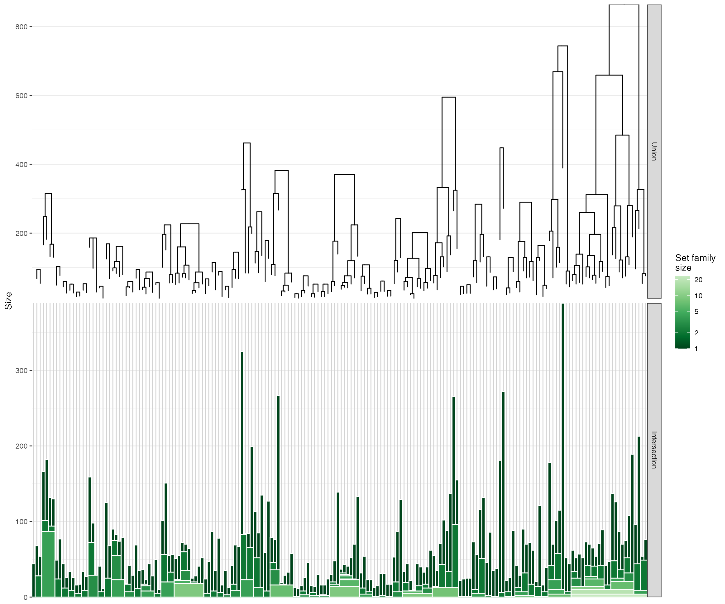
There is clearly a lot of overlap between these genesets…
plot(hierarchy, type='outlyingElements', quantiles=0.75, alpha=0.5, label=FALSE)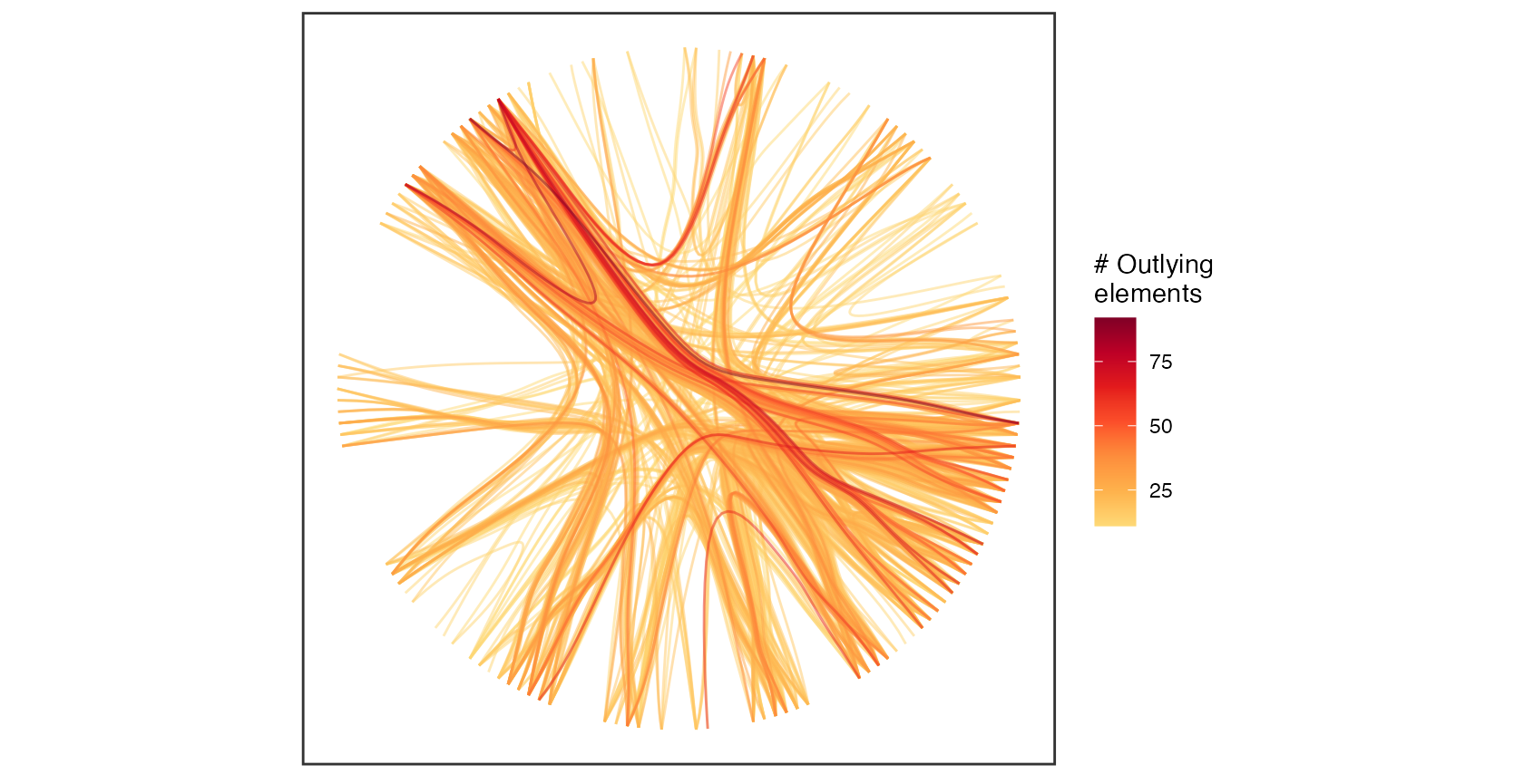
Extracting the hierarchy
suppressPackageStartupMessages(library(dendextend))
suppressPackageStartupMessages(library(stringi))
A helper function for recursively reading and extracting trees from the clustering structure.
find.trees <- function(d) {
    subtrees <- dendextend::partition_leaves(d)
    leaves <- subtrees[[1]]
    find.paths <- function(leaf) {
        which(sapply(subtrees, function(x) leaf %in% x))
    }
    paths <- lapply(leaves, find.paths)
    edges <- data.frame(from=c(), to=c())
    if (length(d) > 1) {
        for (path in paths) {
            for (i in seq(1, length(path)-1)) {
                edges <- rbind(edges, data.frame(from=path[i], to=path[i+1]))
            }
        }
        edges <- dplyr::distinct(edges)
        edges$from <- paste0("N", edges$from)
        edges$to <- paste0("N", edges$to)
    }
    names(subtrees) <- paste0("N", seq(1:length(subtrees)))
    nodes <- data.frame(id=names(subtrees))
    rownames(nodes) <- nodes$id
    nodes$label <- ""
    leaves <- sapply(subtrees, function(x) length(x) == 1)
    nodes$label[leaves] <- sapply(subtrees[leaves], function(x) x[[1]])
    nodes$id <- NULL

    # Internal nodes will not have labels, so we can generate unique hash identifiers
    ids <- stringi::stri_rand_strings(nrow(nodes), 32)
    names(ids) <- rownames(nodes)
    rownames(nodes) <- ids[rownames(nodes)]
    edges$from <- ids[edges$from]
    edges$to <- ids[edges$to]

    return(list("edges"=edges, "nodes"=nodes))
}[1] 50Now we can merge the independent trees into a single graph…
Nodes
                                                                                      label
jUUzOhno3bloMT8QXE5KGQaVvwBRt2K1                                           Abc Transporters
A296wAg1OnK4UfspjYApkvaIEdDMNEcG
ZQmYXCWN7gey2YHYPkyZ2Z2cO5VguNoY Epithelial Cell Signaling In Helicobacter Pylori Infection
Amkon0r1hXwUMAFd5vB1b2kM3iaTqHnO                                  Vibrio Cholerae Infection
cPj5PgqXVbw9o6m48RbiIvWasBMNI7oa
tdqY8vlhyDwxanxeOX0rarojDMsS1Hb9
Edges
edges.all <- lapply(trees, function(x) x$edges)
edges <- data.frame(do.call(rbind, edges.all))
head(edges)
from to
1 A296wAg1OnK4UfspjYApkvaIEdDMNEcG ZQmYXCWN7gey2YHYPkyZ2Z2cO5VguNoY
2 A296wAg1OnK4UfspjYApkvaIEdDMNEcG Amkon0r1hXwUMAFd5vB1b2kM3iaTqHnO
3 cPj5PgqXVbw9o6m48RbiIvWasBMNI7oa tdqY8vlhyDwxanxeOX0rarojDMsS1Hb9
4 tdqY8vlhyDwxanxeOX0rarojDMsS1Hb9 yNMKl6Su7kkPooY2l1WE6SjTGZLYVE4b
5 tdqY8vlhyDwxanxeOX0rarojDMsS1Hb9 zdr2p3XuCE4CbFHRbC78che7tIfiZYNd
6 cPj5PgqXVbw9o6m48RbiIvWasBMNI7oa KsTjbfPIC7orJKNRMF89pm0wCGtXmiDICreate the relational genesets object…
rgsets_obj <- rgsets$new(genesets, nodes, edges, name="MSIGDB_KEGG", version=msigdb_version())
rgsets_objMSIGDB_KEGG v7.2.1
Genesets
Abc Transporters (44)
Acute Myeloid Leukemia (57)
Adherens Junction (73)
Adipocytokine Signaling Pathway (67)
Alanine Aspartate And Glutamate Metabolism (32)
Aldosterone Regulated Sodium Reabsorption (42)
Nodes
label
jUUzOhno3bloMT8QXE5KGQaVvwBRt2K1 Abc Transporters
A296wAg1OnK4UfspjYApkvaIEdDMNEcG
ZQmYXCWN7gey2YHYPkyZ2Z2cO5VguNoY Epithelial Cell Signaling In Helicobacter Pylori Infection
Amkon0r1hXwUMAFd5vB1b2kM3iaTqHnO Vibrio Cholerae Infection
cPj5PgqXVbw9o6m48RbiIvWasBMNI7oa
tdqY8vlhyDwxanxeOX0rarojDMsS1Hb9
id length
jUUzOhno3bloMT8QXE5KGQaVvwBRt2K1 jUUzOhno3bloMT8QXE5KGQaVvwBRt2K1 44
A296wAg1OnK4UfspjYApkvaIEdDMNEcG A296wAg1OnK4UfspjYApkvaIEdDMNEcG 95
ZQmYXCWN7gey2YHYPkyZ2Z2cO5VguNoY ZQmYXCWN7gey2YHYPkyZ2Z2cO5VguNoY 68
Amkon0r1hXwUMAFd5vB1b2kM3iaTqHnO Amkon0r1hXwUMAFd5vB1b2kM3iaTqHnO 54
cPj5PgqXVbw9o6m48RbiIvWasBMNI7oa cPj5PgqXVbw9o6m48RbiIvWasBMNI7oa 315
tdqY8vlhyDwxanxeOX0rarojDMsS1Hb9 tdqY8vlhyDwxanxeOX0rarojDMsS1Hb9 248
Edges
                              from                               to
1 A296wAg1OnK4UfspjYApkvaIEdDMNEcG ZQmYXCWN7gey2YHYPkyZ2Z2cO5VguNoY
2 A296wAg1OnK4UfspjYApkvaIEdDMNEcG Amkon0r1hXwUMAFd5vB1b2kM3iaTqHnO
3 cPj5PgqXVbw9o6m48RbiIvWasBMNI7oa tdqY8vlhyDwxanxeOX0rarojDMsS1Hb9
4 tdqY8vlhyDwxanxeOX0rarojDMsS1Hb9 yNMKl6Su7kkPooY2l1WE6SjTGZLYVE4b
5 tdqY8vlhyDwxanxeOX0rarojDMsS1Hb9 zdr2p3XuCE4CbFHRbC78che7tIfiZYNd
6 cPj5PgqXVbw9o6m48RbiIvWasBMNI7oa KsTjbfPIC7orJKNRMF89pm0wCGtXmiDI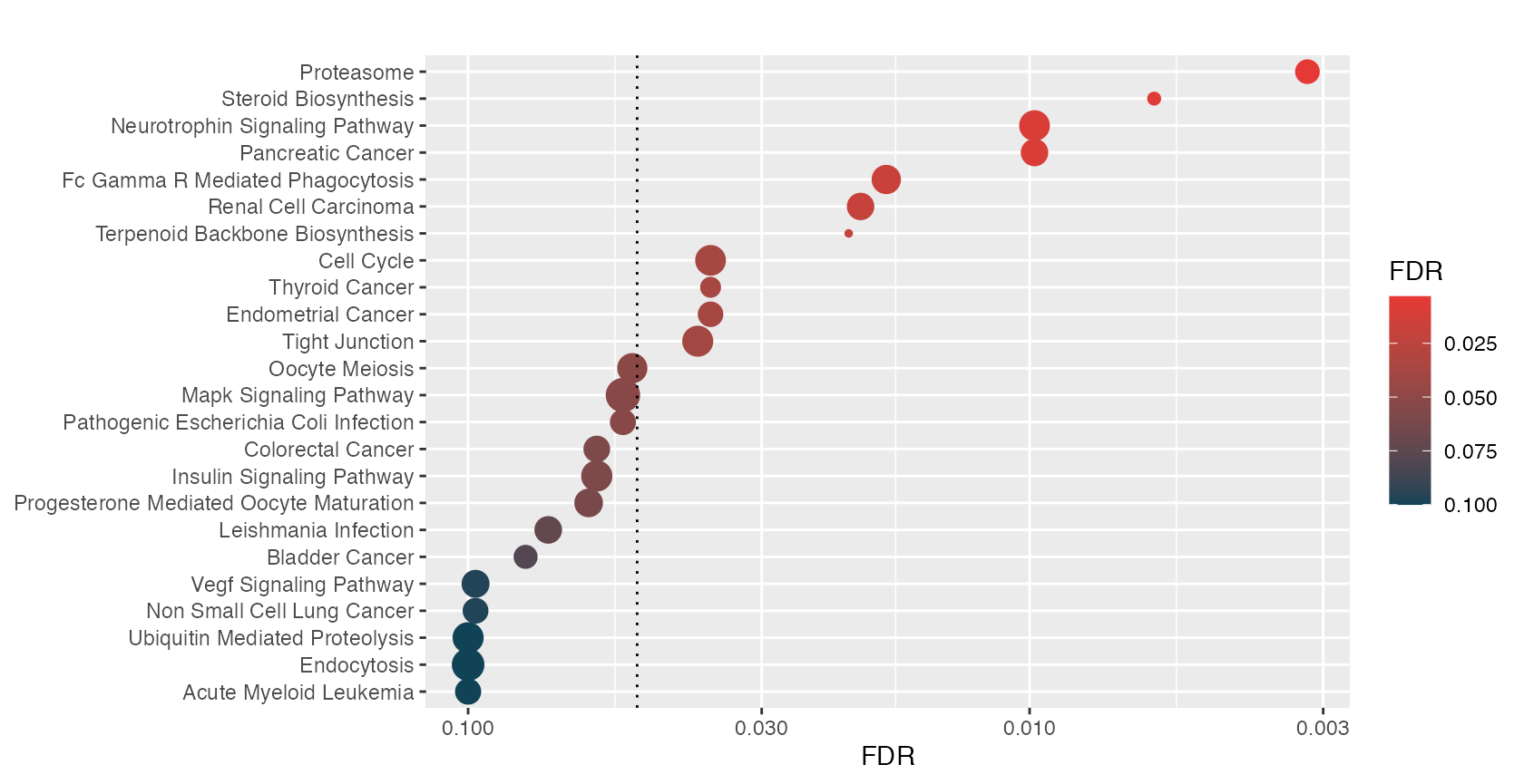
hyp_hmap(hyp, fdr=0.1)