This vignette outlines the workflow for comparing
OmicSignature objects and visualizing similarity among
signatures.
Compare one list of signatures
Use compare_omic_signatures() with a named list of
OmicSignature objects to compare every signature against
every other signature in the list. For bi-directional signatures, the
function compares the first factor level against the first factor level
and the second factor level against the second factor level.
library(OmicSignature)

data(compare_signatures_example)
signature_list <- compare_signatures_example

overlap_res <- compare_omic_signatures(
  sig_list1 = signature_list,
  method = "overlap",
  score_cutoff = log2(1.25),
  adj_p_cutoff = 0.05,
  min_features = 25,
  max_feature = 2000
)
## show the label order
overlap_res$label_order
#> $sig_list1
#>              level1 level2
#> e7386_hsc3   "DMSO" "E7386"
#> e7386_cal27  "DMSO" "E7386"
#> icg001_hsc3  "DMSO" "ICG001"
#> icg001_cal27 "DMSO" "ICG001"

## list the comparisons being performed
names(overlap_res$comparisons)
#> [1] "level1_vs_level1" "level2_vs_level2"

## show the comparison results for level 1 (jaccard and counts)
overlap_res$comparisons$level1_vs_level1$jaccard
#>              e7386_hsc3 e7386_cal27 icg001_hsc3 icg001_cal27
#> e7386_hsc3    1.0000000   0.3023088   0.4600457    0.2535613
#> e7386_cal27   0.3023088   1.0000000   0.2141944    0.2862150
#> icg001_hsc3   0.4600457   0.2141944   1.0000000    0.2384770
#> icg001_cal27  0.2535613   0.2862150   0.2384770    1.0000000

## in the counts matrix, you can see the signature sizes in the diagonal
overlap_res$comparisons$level1_vs_level1$counts
#>              e7386_hsc3 e7386_cal27 icg001_hsc3 icg001_cal27
#> e7386_hsc3         1232         419         806          356
#> e7386_cal27         419         573         335          245
#> icg001_hsc3         806         335        1326          357
#> icg001_cal27        356         245         357          528
The overlap method returns three matrices for each compared factor level:
-
jaccard: Jaccard similarity between retained feature sets. -
pvalue: Fisher exact test p-values for overlap enrichment. -
counts: an integer matrix with the same dimensions asjaccard/pvalue. Entry[i, j]is the overlap size between signatureiand signaturej; for self-comparisons, the diagonal is therefore each signature’s own retained feature-set size.
Compare two lists of signatures
Pass both sig_list1 and sig_list2 to
compare signatures across collections. This is useful when signatures
come from different studies, cohorts, platforms, or perturbation
screens.
reference_signatures <- compare_signatures_example[1:2]
query_signatures <- compare_signatures_example[3:4]

cross_res <- compare_omic_signatures(
  sig_list1 = query_signatures,
  sig_list2 = reference_signatures,
  method = "overlap",
  score_cutoff = log2(1.25),
  adj_p_cutoff = 0.05,
  min_features = 25,
  max_feature = 500
)

cross_res$comparisons$level1_vs_level1$jaccard
#>              e7386_hsc3 e7386_cal27
#> icg001_hsc3   0.2048193   0.1415525
#> icg001_cal27  0.2437811   0.2804097
When background is not supplied, the feature universe is
inferred from all available signature and differential-expression tables
in both inputs. Supplying a measured or assay-specific background is
recommended when it is available.
Control label pairing
By default, level ordering follows the factor levels in each
signature’s group_label column. Use
label_pairing and label_pairing2 when
signatures need explicit matching.
data(compare_label_pairing_example)

## let's see the order of the signatures' group_label's
compare_label_pairing_example |>
  sapply(\(x) levels(x$difexp$group_label)) |> t() |>
  as.data.frame() |> setNames(c("level1", "level2"))
#>                level1    level2
#> signature_a   treated   control
#> signature_b      down        up
#> signature_c resistant sensitive

## compare signatures and provide the desired label pairing
paired_res <- compare_omic_signatures(
  sig_list1 = compare_label_pairing_example,
  method = "overlap",
  label_pairing = list(
    signature_a = c("treated", "control"),
    signature_b = c("up", "down"),
    signature_c = c("resistant", "sensitive")
  )
)
## level1 vs. level1
paired_res$comparisons$level1_vs_level1$jaccard
#>             signature_a signature_b signature_c
#> signature_a   1.0000000   0.6666667   0.3333333
#> signature_b   0.6666667   1.0000000   0.3333333
#> signature_c   0.3333333   0.3333333   1.0000000

## level2 vs. level2
paired_res$comparisons$level2_vs_level2$jaccard
#>             signature_a signature_b signature_c
#> signature_a   1.0000000   0.6666667   0.3333333
#> signature_b   0.6666667   1.0000000   0.3333333
#> signature_c   0.3333333   0.3333333   1.0000000
KS and GSEA-style comparisons
The ks_rank, ks_score, and
gsea methods compare a retained feature set from one
signature against ranked differential-expression scores from another
signature. These methods require the compared OmicSignature
objects to retain their difexp tables. For each requested
group_label, genes are ranked from the largest
-log10(p_value) in that label to the largest
-log10(p_value) in the contrasting label.
ks_rank tests where the retained features fall in that
ranking, while ks_score compares their numeric ranking
scores against the remaining features. The legacy
method = "ks" name is accepted as an alias for
method = "ks_rank".
ks_res <- compare_omic_signatures(
  sig_list1 = signature_list,
  method = "ks_rank",
  adj_p_cutoff = 0.05,
  min_features = 25,
  max_feature = 500
)

ks_res$comparisons$level1_vs_level1$score
#>              e7386_hsc3 e7386_cal27 icg001_hsc3 icg001_cal27
#> e7386_hsc3    0.8592342   0.4160968   0.4107636    0.4287572
#> e7386_cal27   0.4201126   0.8589527   0.3174991    0.4384881
#> icg001_hsc3   0.4059002   0.3219889   0.8509243    0.4114431
#> icg001_cal27  0.4019190   0.4744036   0.3374776    0.8509243
ks_res$comparisons$level1_vs_level1$pvalue
#>              e7386_hsc3 e7386_cal27 icg001_hsc3 icg001_cal27
#> e7386_hsc3            0           0           0            0
#> e7386_cal27           0           0           0            0
#> icg001_hsc3           0           0           0            0
#> icg001_cal27          0           0           0            0
The simulated label-pairing data can also be compared with
ks_score. In this toy example, the treated/up/resistant
labels define the first level and the control/down/sensitive labels
define the second level.
toy_ks_score <- compare_omic_signatures(
  sig_list1 = compare_label_pairing_example,
  method = "ks_score",
  label_pairing = list(
    signature_a = c("treated", "control"),
    signature_b = c("up", "down"),
    signature_c = c("resistant", "sensitive")
  ),
  min_features = 5
)

round(toy_ks_score$comparisons$level1_vs_level1$score, 3)
#>             signature_a signature_b signature_c
#> signature_a         1.0         0.8       0.556
#> signature_b         0.8         1.0       0.556
#> signature_c         0.5         0.5       1.000

signif(toy_ks_score$comparisons$level1_vs_level1$pvalue, 3)
#>             signature_a signature_b signature_c
#> signature_a    5.78e-14    2.83e-10    6.24e-04
#> signature_b    2.83e-10    5.78e-14    6.24e-04
#> signature_c    1.03e-03    3.44e-05    5.78e-14

round(toy_ks_score$comparisons$level2_vs_level2$score, 3)
#>             signature_a signature_b signature_c
#> signature_a         1.0         0.8         0.5
#> signature_b         0.8         1.0         0.5
#> signature_c         0.5         0.5         1.0

signif(toy_ks_score$comparisons$level2_vs_level2$pvalue, 3)
#>             signature_a signature_b signature_c
#> signature_a    5.78e-14    2.83e-10    6.27e-04
#> signature_b    2.83e-10    5.78e-14    6.27e-04
#> signature_c    3.44e-05    1.61e-03    5.78e-14
GSEA requires the optional fgsea package.
gsea_res <- compare_omic_signatures(
  sig_list1 = signature_list,
  method = "gsea",
  adj_p_cutoff = 0.05,
  min_features = 25,
  max_feature = 500,
  minSize = 10,
  maxSize = 500
)
Plot similarity heatmaps
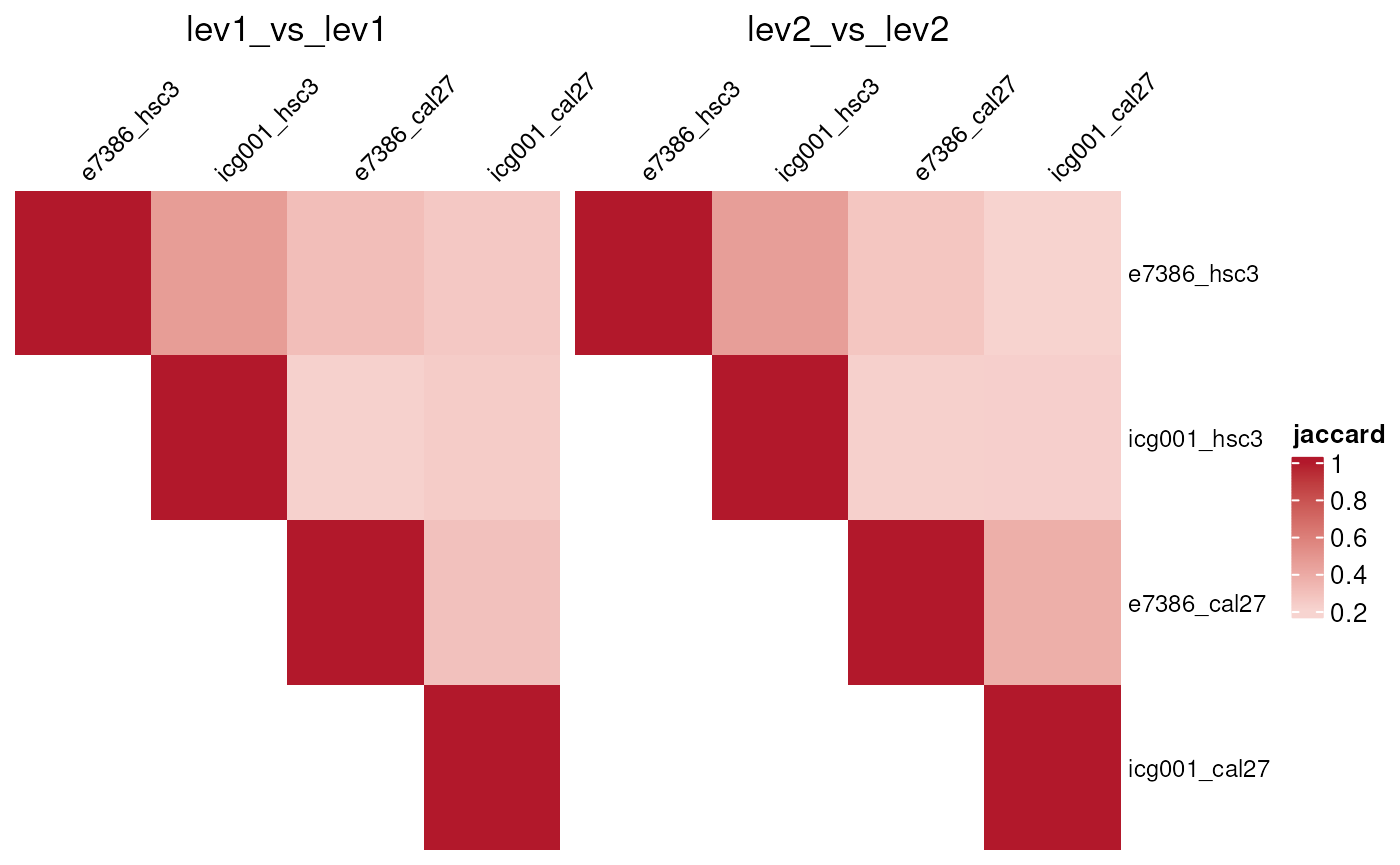
Use signature_similarity_heatmap() to visualize square
self-comparison output from
compare_omic_signatures(method = "overlap"). The heatmap
function requires the optional ComplexHeatmap and
circlize packages.
signature_similarity_heatmap(
  overlap_res,
  measure = "jaccard",
  mode = "separate",
  triangle = "upper",
  column_names_gp = grid::gpar(fontsize = 9),
  row_names_gp = grid::gpar(fontsize = 9),
  column_names_rot = 45
)
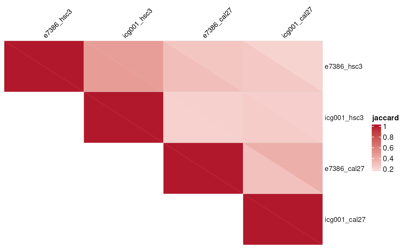
With mode="combined", a single triangular matrix is
shown, with each entry divided into two triangles displaying the level2
(top-right) and level1 (bottom-left) similarity.
signature_similarity_heatmap(
  overlap_res,
  measure = "jaccard",
  mode = "combined",
  triangle = "upper",
  column_names_gp = grid::gpar(fontsize = 9),
  row_names_gp = grid::gpar(fontsize = 9),
  column_names_rot = 45
)
For measure = "pvalue", values are plotted as
-log10(pvalue). Larger values therefore indicate stronger
overlap enrichment.
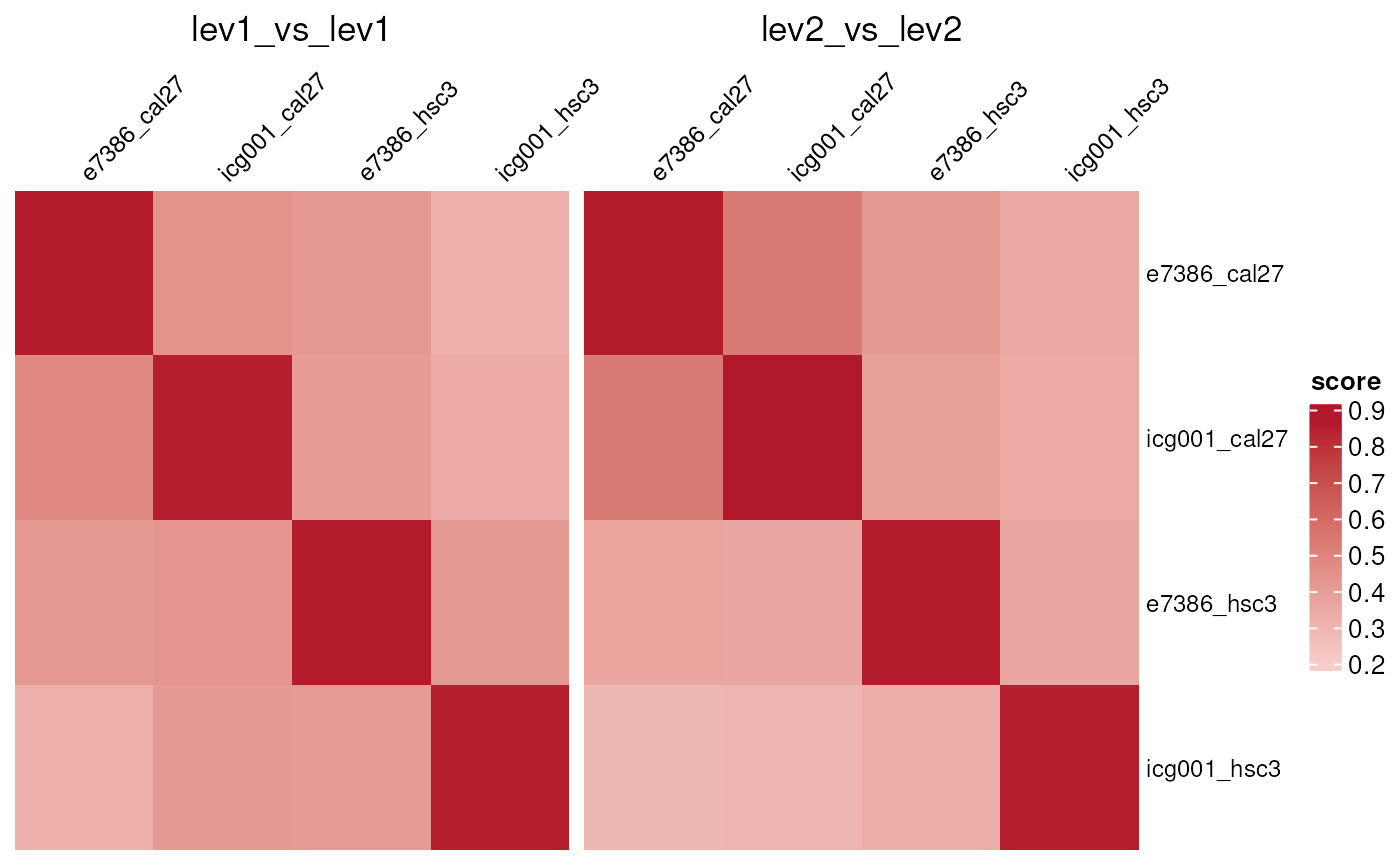
Rank-based KS and GSEA outputs can be visualized with
measure = "score" or measure = "pvalue".
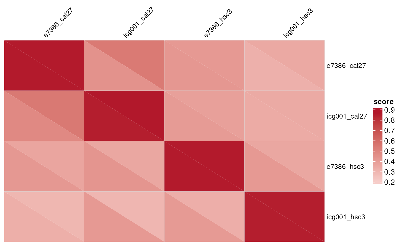
Because these matrices are directional rather than symmetric,
mode = "combined" draws the full square matrix (not just
one triangle), splitting each cell into two triangles that superimpose
the two mode = "separate" matrices: the bottom-left
triangle shows level1_vs_level1 and the top-right triangle
shows level2_vs_level2. mode = "separate"
draws those same two matrices as separate, full heatmaps instead.
signature_similarity_heatmap(
  ks_res,
  measure = "score",
  mode = "combined",
  triangle = "upper",
  column_names_gp = grid::gpar(fontsize = 9),
  row_names_gp = grid::gpar(fontsize = 9),
  column_names_rot = 45
)
signature_similarity_heatmap(
  ks_res,
  measure = "score",
  mode = "separate",
  column_names_gp = grid::gpar(fontsize = 9),
  row_names_gp = grid::gpar(fontsize = 9),
  column_names_rot = 45
)