Data Example

Example dataset

To get a sense of how this works, there is a simulated network with modular scale-free properties available. The object already has pre-defined communities that have been populated with genes from highly specific biological pathways. This data was generated through the following steps:

1. Simulate a graph structure through the Lancichinetti–Fortunato–Radicchi (LFR) benchmark model
2. Detect and define communities within the graph
3. For each community sample node labels from a biological pathway (80%) / random (20%)

LFR(n=600, tau1=2.7, tau2=2, mu=0.1, min_community=25, max_community=75)

data(ig)

This package works with undirected igraph objects or extensions of igraph objects.

is(ig)

[1] "igraph"

set.seed(1)
layout <- igraph::layout_with_graphopt(ig, 
                                       start=NULL, 
                                       niter=1000,
                                       charge=0.005,
                                       mass=30, 
                                       spring.length=0,
                                       spring.constant=1, 
                                       max.sa.movement=5)

par(mar=c(0,0,0,0))
plot(ig,
     vertex.size=4,
     vertex.color="#EEEEEE",
     vertex.frame.color=adjustcolor("#000000", alpha.f=0.2),
     vertex.label=V(ig)$symbol,
     vertex.label.family="Helvetica",
     vertex.label.color="black",
     vertex.label.font=2,
     vertex.label.cex=0.4,
     vertex.label.dist=0,
     edge.width=1,
     layout=layout)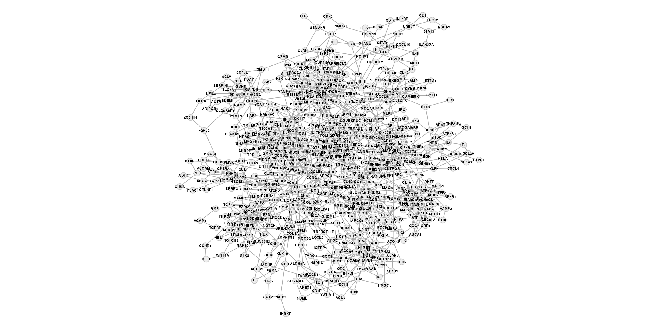

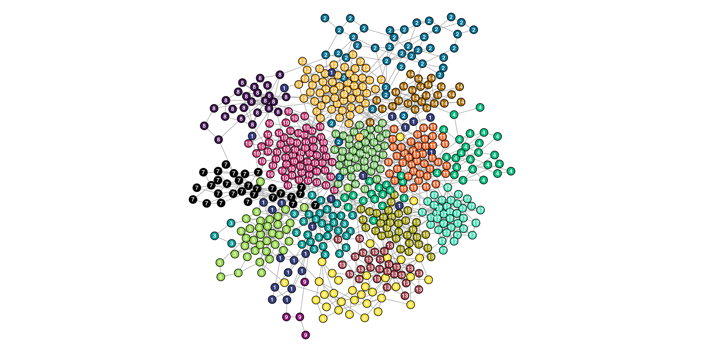
You need to perform some type of community detection. There are many algorithms but I prefer defining community structure through random walks. Walktrap looks for densely connected subgraphs through random walks at varying lengths. Whatever algorithm you use, make sure to label the nodes with their designated community through V(ig)$community.

set.seed(1)
ig.c <- igraph::walktrap.community(ig, steps=10)
V(ig)$community <- ig.c$membership

table(V(ig)$community)

 1  2  3  4  5  6  7  8  9 10 11 12 13 14 15 16 17 
24 42 33 41 37 34 29 25  4 66 43 55 27 26 33 45 36 

The following vertex attributes are expected at a minimum.

• name - Unique node labels
• symbol - Node symbols corresponding to the genesets you use
  
• community- Pre-detected community labels
  
• color - Community-specific colors

head(igraph::as_data_frame(ig, what="vertices"))

       community   color symbol   name
GMPS           8 #3E134F   GMPS   GMPS
PDLIM1        15 #9A9800 PDLIM1 PDLIM1
JUNB          15 #9A9800   JUNB   JUNB
RER1          17 #50E2BB   RER1   RER1
ICAM1         14 #A96C00  ICAM1  ICAM1
NPFFR2        14 #A96C00 NPFFR2 NPFFR2

We can visualize the communities which seem well-defined. Not surprisingly since this example data was defined to be particularly modular for demonstration purposes.

par(mar=c(0,0,0,0))
plot(ig,
     vertex.size=5,
     vertex.label=V(ig)$community,
     vertex.label.family="Helvetica",
     vertex.label.color="white",
     vertex.label.font=2,
     vertex.label.cex=0.6,
     vertex.label.dist=0,
     edge.width=1,
     layout=layout)