Markov Networks-based Differential Connectivity Analysis

Introduction

Differential connectivity analysis is an important application in network-based studies, aimed at characterizing network rewiring patterns of interacting entities across different conditions or phenotypes. Unlike univariate analyses that evaluate features independently, this approach captures integrative, system-level signals arising from the collective behavior of interacting entities, thereby providing complementary insights into underlying mechanisms.

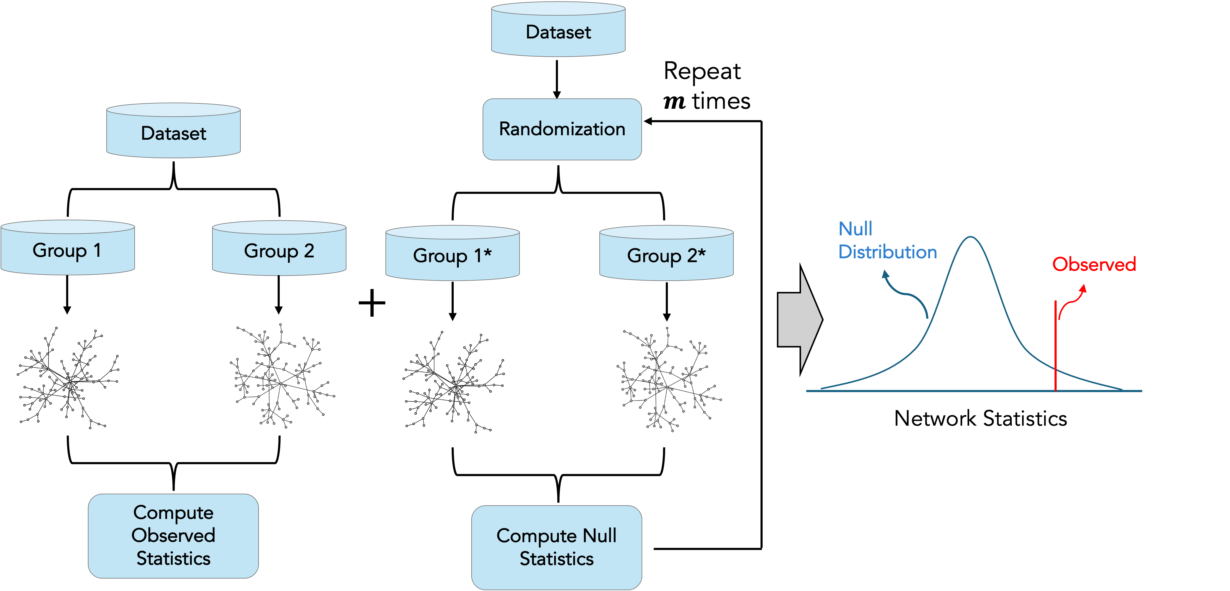
RSNet supports differential connectivity analysis for datasets containing samples from two groups (e.g., young vs. old, disease vs. healthy) and enables statistical assessment of a wide range of network-based statistics, including centrality measures and graphlet degree vector (GDV)–based distances.The overall workflow is illustrated in the following figure. Briefly, the input dataset is partitioned into two mutually exclusive subsets corresponding to the groups of interest. Network structure inference is then performed separately for each subset, and the observed differences in network-based statistics are computed.

To assess statistical significance, RSNet constructs a resampling-based empirical null distribution by randomizing the original dataset using permutation and/or bootstrap procedures. The significance of the observed network differences is subsequently evaluated by comparing the observed statistics to the corresponding null distributions.

Load packages

library(RSNet)
library(igraph)
library(DT)

Load LOAD dataset

Here, we use a curated dataset derived from a late-onset Alzheimer’s disease (LOAD) study.

Here we used a real, and curated dataset derived from late-onset Alzheimer’s disease (LOAD) study. The dataset includes 129 LOAD subjects and 101 control subjects. For demonstration and computational efficiency, we use only a subset of genes with the highest median absolute deviation (MAD).

data(toy_load)

Estimate observed networks

The observed networks are constructed by splitting the dataset into two groups based on the phenotype of interest, LOAD versus Control. Each subset of the data is then used as input to the resampling-based framework implemented in RSNet. The resulting networks derived from each group are stored as a named list object for downstream analyses.

## split the data into two groups
ctrl_dat <- toy_load %>% 
  dplyr::filter(phenotype == "ctrl") %>% 
  dplyr::select(-phenotype)

load_dat <- toy_load %>% 
  dplyr::filter(phenotype == "load") %>% 
  dplyr::select(-phenotype)


## Infer observed networks from each group
ctrl_obs <- capture_all(ensemble_ggm(dat = ctrl_dat,
                         num_iteration = 1,
                         sub_ratio = 1,
                         method = "D-S_NW_SL",
                         n_cores = 1)) %>% 
  consensus_net_ggm(., filter = "pval", threshold = 0.05) %>% 
  { .[["consensus_network"]] }

load_obs <- capture_all(ensemble_ggm(dat = load_dat,
                         num_iteration = 1,
                         sub_ratio = 1,
                         method = "D-S_NW_SL",
                         n_cores = 1)) %>% 
  consensus_net_ggm(., filter = "pval", threshold = 0.05) %>% 
  { .[["consensus_network"]] }


## Create a list of observed networks
obs_networks <- list(ctrl = ctrl_obs,
                     load = load_obs)

Estimate the null distribution

Accurate estimation of the null distribution is essential for assessing statistical significance. owever, for most network-based statistics, the null distribution is difficult to derive analytically. RSNet addresses this challenge by implementing resampling-based null distribution generation via permutation and bootstrap methods. These procedures are implemented in the null_ggm() function.

Because null generation can be computationally intensive, null_ggm() also supports parallel computing for improved efficiency.

In the following example, we generate two null distributions, one using permutation and one using bootstrap, each with five iterations.

shuffle_iter <- 5

null_permutation <- capture_all(null_ggm(dat = toy_load, # a n x (p+1) data frame with p numeric feature columns + one label column.
                             group_col = "phenotype", # name of the label (phenotype) column
                             inference_method = "D-S_NW_SL", # the inference method
                             shuffle_method = "permutation", # shuffling method
                             shuffle_iter = shuffle_iter, # number of iteration
                             filter = "pval", # filter criteria, support "pval", "fdr", and "none"
                             threshold = 0.05, # the significance level
                             n_cores = 1)) # number of cores for parallel computing

null_bootstrap <- capture_all(null_ggm(dat = toy_load,
                           group_col = "phenotype",
                           inference_method = "D-S_NW_SL",
                           shuffle_method = "bootstrap",
                           shuffle_iter = shuffle_iter,
                           filter = "pval",
                           threshold = 0.05,
                           n_cores = 1))

## A list of length "shuffle_iter"; each element is a named list (by group labels) of igraph objects
stopifnot(length(null_permutation$null_networks) == shuffle_iter)
stopifnot(length(null_bootstrap$null_networks) == shuffle_iter)

Differential centralities

RSNet supports differential analysis of standard centrality measures, including degree, eigenvector, and betweenness centralities, etc. This functionality is implemented in the diff_centrality() function, which takes as input the observed networks。

Internally, diff_centrality() calls the null_ggm() function to generate the null distribution. For improved memory efficiency, users can alternatively run null_ggm() separately and supply its output to the null_networks argument.

The diff_centrality() function supports both permutation-based and bootstrap-based randomization procedures, and allows for one-sided or two-sided hypothesis testing.

diff_centrality_res <- capture_all(diff_centrality(obs_networks = obs_networks,
                                       dat = toy_load,
                                       group_col = "phenotype",
                                       null_networks = NULL,
                                       alternative = "two.sided",
                                       inference_method = "D-S_NW_SL",
                                       shuffle_method = "permutation",
                                       shuffle_iter = 5,
                                       balanced = FALSE,
                                       filter = "pval",
                                       threshold = 0.05,
                                       n_cores =  1,
                                       seed = 42))

diff_centrality_res %>% 
  head(.) %>% 
  DT::datatable(.)

Differential graphlet degree vector(GDV)-based distance

In addition to differential analysis of standard centrality measures, RSNet also supports graphlet degree vector (GDV)-based distance analysis (see the Graphlet page for details). This functionality is implemented in the diff_gdv() function.

The arguments of diff_gdv() are similar to those of diff_centrality(). However, diff_gdv() currently supports only permutation-based randomization procedures and performs one-sided hypothesis testing, consistent with the statistical characteristics of the GDV distance measure.

diff_gdv_res <- capture_all(diff_gdv(obs_networks = obs_networks,
                         dat = toy_load,
                         group_col = "phenotype",
                         null_networks = NULL,
                         sign = TRUE,
                         inference_method = "D-S_NW_SL",
                         shuffle_method = "permutation",
                         shuffle_iter = 5,
                         balanced = FALSE,
                         filter = "pval",
                         threshold = 0.05,
                         n_cores =  1,
                         seed = 42))

diff_gdv_res %>% 
  head(.) %>% 
  DT::datatable(.)

Ziwei Huang