The CaDrA package currently supports four scoring functions to search for subsets of genomic features that are likely associated with a specific outcome of interest (e.g., protein expression, pathway activity, etc.)
- Kolmogorov-Smirnov Method (
ks) - Wilcoxon Rank-Sum Method (
wilcox) - Conditional Mutual Information Method (
revealer) - K-Nearest Neighbor Mutual Information Estimator
(
knnmi) - Correlation Method (
correlation) - Custom - An User Defined Scoring Method (
custom)
Below, we run candidate_search() over the top 3 starting
features using each of the scoring functions described above.
Important Notes:
- The legacy or deprecated function
topn_eval()is equivalent to the new and recommendedcandidate_search()function
Load packages
library(CaDrA)
library(pheatmap)
library(SummarizedExperiment)
Load required datasets
- A
binary features matrixalso known asFeature Set(such as somatic mutations, copy number alterations, chromosomal translocations, etc.) The 1/0 row vectors indicate the presence/absence of ‘omics’ features in the samples. TheFeature Setcan be a matrix or an object of class SummarizedExperiment from SummarizedExperiment package) - A vector of continuous scores (or
Input Scores) representing a functional response of interest (such as protein expression, pathway activity, etc.)
Heatmap of simulated feature set
The simulated dataset, sim_FS, comprises of 1000 genomic
features and 100 sample profiles. There are 10 left-skewed (i.e. True
Positive or TP) and 990 uniformly-distributed (i.e. True Null or TN)
features simulated in the dataset. Below is a heatmap of the first 100
features.
mat <- SummarizedExperiment::assay(sim_FS)
pheatmap::pheatmap(mat[1:100, ], color = c("white", "red"), cluster_rows = FALSE, cluster_cols = FALSE)
Search for a subset of genomic features that are likely associated with a functional response of interest using each of the scoring methods
1. Kolmogorov-Smirnov Scoring Method
See ?ks_rowscore for more details
ks_topn_l <- CaDrA::candidate_search(
  FS = sim_FS,
  input_score = sim_Scores,
  method = "ks_pval",          # Use Kolmogorov-Smirnov scoring function
  method_alternative = "less", # Use one-sided hypothesis testing
  weights = NULL,              # If weights is provided, perform a weighted-KS test
  search_method = "both",      # Apply both forward and backward search
  top_N = 3,                   # Evaluate top 3 starting points for the search
  max_size = 10,               # Allow at most 10 features in meta-feature matrix
  do_plot = FALSE,             # We will plot it AFTER finding the best hits
  best_score_only = FALSE      # Return all results from the search
)

# Now we can fetch the feature set of top N features that corresponded to the best scores over the top N search
ks_topn_best_meta <- topn_best(ks_topn_l)

# Visualize best meta-feature result
meta_plot(topn_best_list = ks_topn_best_meta)
2. Wilcoxon Rank-Sum Scoring Method
See ?wilcox_rowscore for more details
wilcox_topn_l <- CaDrA::candidate_search(
  FS = sim_FS,
  input_score = sim_Scores,
  method = "wilcox_pval",      # Use Wilcoxon Rank-Sum scoring function
  method_alternative = "less", # Use one-sided hypothesis testing
  search_method = "both",      # Apply both forward and backward search
  top_N = 3,                   # Evaluate top 3 starting points for the search
  max_size = 10,               # Allow at most 10 features in meta-feature matrix
  do_plot = FALSE,             # We will plot it AFTER finding the best hits
  best_score_only = FALSE      # Return all results from the search
)

# Now we can fetch the feature set of top N feature that corresponded to the best scores over the top N search
wilcox_topn_best_meta <- topn_best(topn_list = wilcox_topn_l)

# Visualize best meta-feature result
meta_plot(topn_best_list = wilcox_topn_best_meta)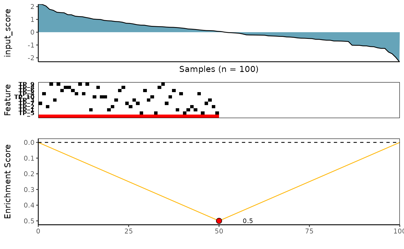
3. Conditional Mutual Information Scoring Method from REVEALER
See ?revealer_rowscore for more details
revealer_topn_l <- CaDrA::candidate_search(
  FS = sim_FS,
  input_score = sim_Scores,
  method = "revealer",         # Use REVEALER's CMI scoring function
  search_method = "both",      # Apply both forward and backward search
  top_N = 3,                   # Evaluate top 3 starting points for the search
  max_size = 10,               # Allow at most 10 features in meta-feature matrix
  do_plot = FALSE,             # We will plot it AFTER finding the best hits
  best_score_only = FALSE      # Return all results from the search
)

# Now we can fetch the ESet of top feature that corresponded to the best scores over the top N search
revealer_topn_best_meta <- topn_best(topn_list = revealer_topn_l)

# Visualize best meta-feature result
meta_plot(topn_best_list = revealer_topn_best_meta)
4. K-Nearest Neighbor Mutual Information Estimator from knnmi package
See ?knnmi_rowscore for more details
knnmi_topn_l <- CaDrA::candidate_search(
  FS = sim_FS,
  input_score = sim_Scores,
  method = "knnmi",            # Use knnmi scoring function
  search_method = "both",      # Apply both forward and backward search
  top_N = 3,                   # Evaluate top 3 starting points for the search
  max_size = 10,               # Allow at most 10 features in meta-feature matrix
  do_plot = FALSE,             # We will plot it AFTER finding the best hits
  best_score_only = FALSE      # Return all results from the search
)

# Now we can fetch the ESet of top feature that corresponded to the best scores over the top N search
knnmi_topn_best_meta <- topn_best(topn_list = knnmi_topn_l)

# Visualize best meta-feature result
meta_plot(topn_best_list = knnmi_topn_best_meta)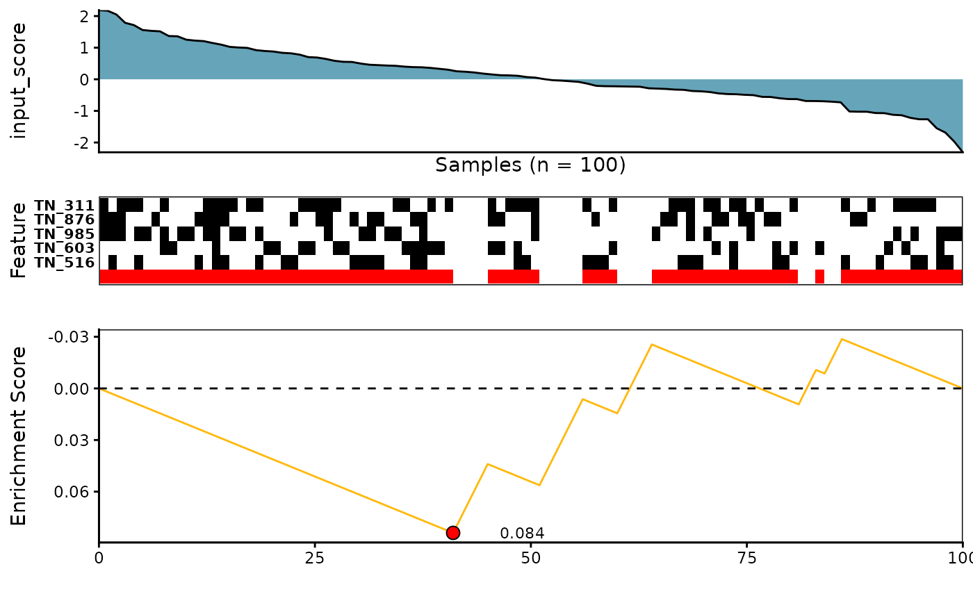
5. Correlation Scoring Method
See ?corr_rowscore for more details
corr_topn_l <- CaDrA::candidate_search(
  FS = SummarizedExperiment::assay(sim_FS),
  input_score = sim_Scores,
  method = "correlation",      # Use correlation scoring function
  cmethod = "spearman",        # Use spearman correlation scoring function
  top_N = 3,                   # Evaluate top 3 starting points for the search
  max_size = 10,               # Allow at most 10 features in meta-feature matrix
  do_plot = FALSE,             # We will plot it AFTER finding the best hits
  best_score_only = FALSE      # Return all results from the search
)

# Now we can fetch the feature set of top N feature that corresponded to the best scores over the top N search
corr_topn_best_meta <- topn_best(topn_list = corr_topn_l)

# Visualize best meta-feature result
meta_plot(topn_best_list = corr_topn_best_meta)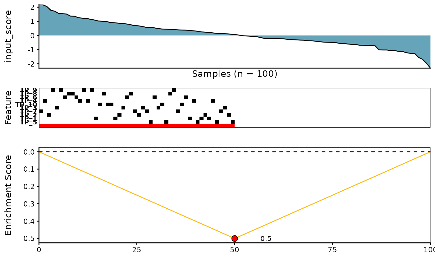
6. Custom - An User Defined Scoring Method
See ?custom_rowscore for more details
# A customized function using ks-test
customized_ks_rowscore <- function(FS, input_score, weights=NULL, meta_feature=NULL, alternative="less", metric="pval"){

  metric <- match.arg(metric)
  alternative <- match.arg(alternative)

  # Check if meta_feature is provided
  if(!is.null(meta_feature)){
    # Getting the position of the known meta features
    locs <- match(meta_feature, row.names(FS))

    # Taking the union across the known meta features
    if(length(locs) > 1) {
      meta_vector <- as.numeric(ifelse(colSums(FS[locs,]) == 0, 0, 1))
    }else{
      meta_vector <- as.numeric(FS[locs, , drop=FALSE])
    }

    # Remove the meta features from the binary feature matrix
    # and taking logical OR btw the remaining features with the meta vector
    FS <- base::sweep(FS[-locs, , drop=FALSE], 2, meta_vector, `|`)*1

    # Check if there are any features that are all 1s generated from
    # taking the union between the matrix
    # We cannot compute statistics for such features and thus they need
    # to be filtered out
    if(any(rowSums(FS) == ncol(FS))){
      verbose("Features with all 1s generated from taking the matrix union ",
              "will be removed before progressing...\n")
      FS <- FS[rowSums(FS) != ncol(FS), , drop=FALSE]
      # If no features remained after filtering, exist the function
      if(nrow(FS) == 0) return(NULL)
    }
  }

  # KS is a ranked-based method
  # So we need to sort input_score from highest to lowest values
  input_score <- sort(input_score, decreasing=TRUE)

  # Re-order the matrix based on the order of input_score
  FS <- FS[, names(input_score), drop=FALSE]

  # Check if weights is provided
  if(length(weights) > 0){
    # Check if weights has any labels or names
    if(is.null(names(weights)))
      stop("The weights object must have names or labels that ",
           "match the labels of input_score\n")

    # Make sure its labels or names match the
    # the labels of input_score
    weights <- as.numeric(weights[names(input_score)])
  }

  # Get the alternative hypothesis testing method
  alt_int <- switch(alternative, two.sided=0L, less=1L, greater=-1L, 1L)

  # Compute the ks statistic and p-value per row in the matrix
  ks <- .Call(ks_genescore_mat_, FS, weights, alt_int)

  # Obtain score statistics from KS method
  # Change values of 0 to the machine lowest value to avoid taking -log(0)
  stat <- ks[1,]

  # Obtain p-values from KS method
  # Change values of 0 to the machine lowest value to avoid taking -log(0)
  pval <- ks[2,]
  pval[which(pval == 0)] <- .Machine$double.xmin

  # Compute the scores according to the provided metric
  scores <- ifelse(rep(metric, nrow(FS)) %in% "pval", -log(pval), stat)
  names(scores) <- rownames(FS)

  return(scores)

}

# Search for best features using a custom-defined function
custom_topn_l <- CaDrA::candidate_search(
  FS = SummarizedExperiment::assay(sim_FS),
  input_score = sim_Scores,
  method = "custom",                        # Use custom scoring function
  custom_function = customized_ks_rowscore, # Use a customized scoring function
  custom_parameters = NULL,                 # Additional parameters to pass to custom_function
  weights = NULL,                           # If weights is provided, perform a weighted test
  search_method = "both",                   # Apply both forward and backward search
  top_N = 3,                                # Evaluate top 3 starting points for the search
  max_size = 10,                            # Allow at most 10 features in meta-feature matrix
  do_plot = FALSE,                          # We will plot it AFTER finding the best hits
  best_score_only = FALSE                   # Return all results from the search
)

# Now we can fetch the feature set of top N feature that corresponded to the best scores over the top N search
custom_topn_best_meta <- topn_best(topn_list = custom_topn_l)

# Visualize best meta-feature result
CaDrA::meta_plot(topn_best_list = custom_topn_best_meta)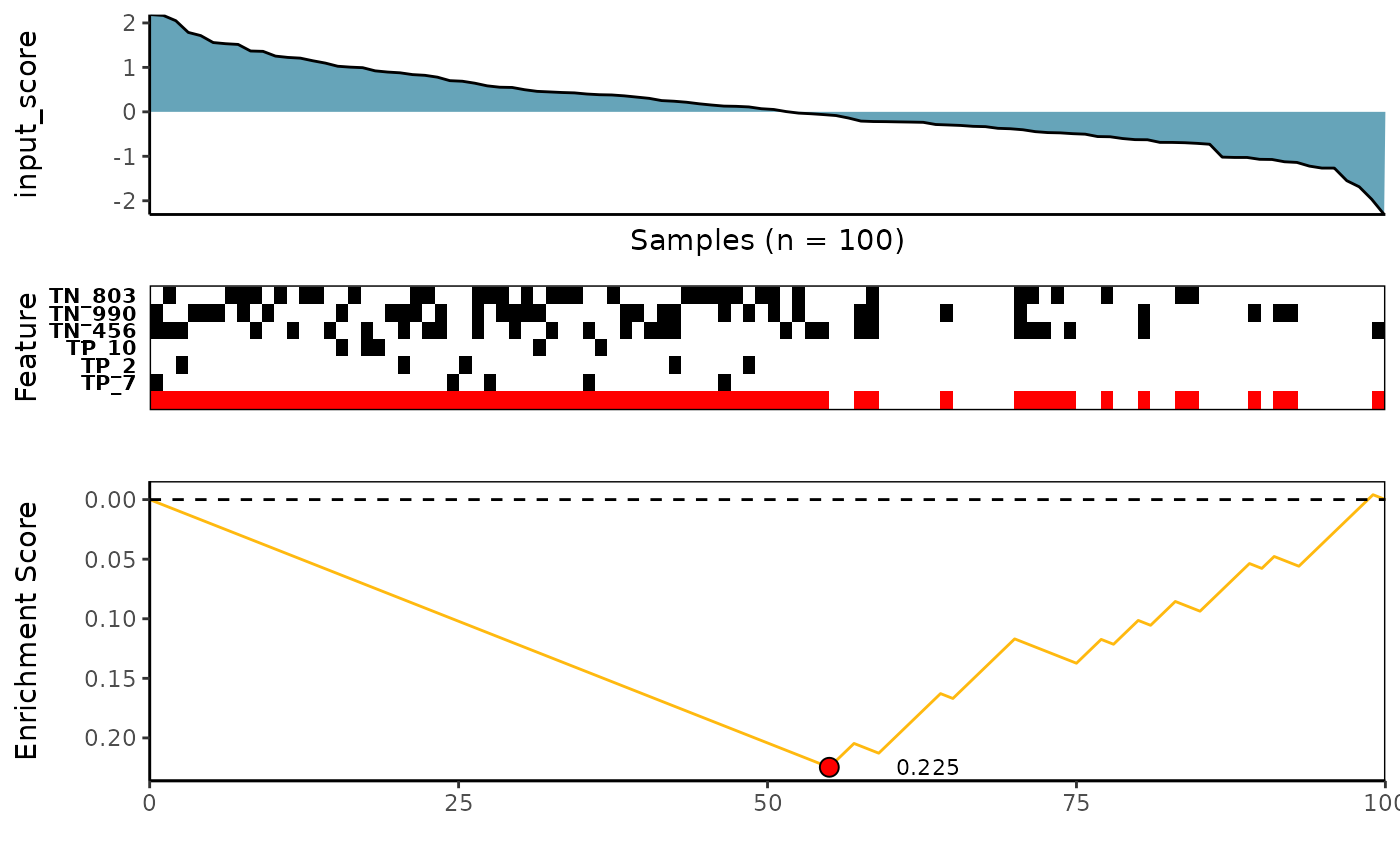
# Evaluate results across top N features you started from
CaDrA::topn_plot(custom_topn_l) 
For validation purposes, compare the custom and built-in function.
topn_res <- CaDrA::candidate_search(
  FS = sim_FS,
  input_score = sim_Scores,
  method = "ks_pval",          # Use Kolmogorov-Smirnov scoring function
  method_alternative = "less", # Use one-sided hypothesis testing
  weights = NULL,              # If weights is provided, perform a weighted-KS test
  search_method = "both",      # Apply both forward and backward search
  top_N = 3,                   # Evaluate top 7 starting points for each search
  max_size = 10,               # Maximum size a meta-feature matrix can extend to
  do_plot = FALSE,             # Plot after finding the best features
  best_score_only = FALSE      # Return all results from the search
)

## Fetch the meta-feature set corresponding to its best scores over top N features searches
topn_best_meta <- topn_best(topn_res)

# Visualize the best results with the meta-feature plot
meta_plot(topn_best_list = topn_best_meta)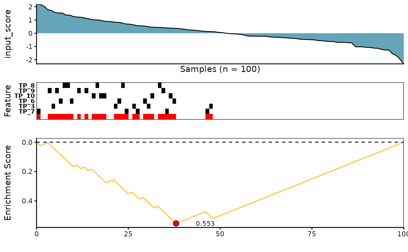
# Evaluate results across top N features you started from
topn_plot(topn_res) 
SessionInfo
sessionInfo()
R version 4.5.1 (2025-06-13)
Platform: x86_64-pc-linux-gnu
Running under: Ubuntu 24.04.3 LTS

Matrix products: default
BLAS:   /usr/lib/x86_64-linux-gnu/openblas-pthread/libblas.so.3
LAPACK: /usr/lib/x86_64-linux-gnu/openblas-pthread/libopenblasp-r0.3.26.so;  LAPACK version 3.12.0

locale:
 [1] LC_CTYPE=C.UTF-8       LC_NUMERIC=C           LC_TIME=C.UTF-8
 [4] LC_COLLATE=C.UTF-8     LC_MONETARY=C.UTF-8    LC_MESSAGES=C.UTF-8
 [7] LC_PAPER=C.UTF-8       LC_NAME=C              LC_ADDRESS=C
[10] LC_TELEPHONE=C         LC_MEASUREMENT=C.UTF-8 LC_IDENTIFICATION=C

time zone: UTC
tzcode source: system (glibc)

attached base packages:
[1] stats4    stats     graphics  grDevices utils     datasets  methods
[8] base

other attached packages:
 [1] CaDrA_1.7.0                 testthat_3.2.3
 [3] devtools_2.4.6              usethis_3.2.1
 [5] pheatmap_1.0.13             SummarizedExperiment_1.38.1
 [7] Biobase_2.68.0              GenomicRanges_1.60.0
 [9] GenomeInfoDb_1.44.3         IRanges_2.42.0
[11] S4Vectors_0.46.0            BiocGenerics_0.54.0
[13] generics_0.1.4              MatrixGenerics_1.20.0
[15] matrixStats_1.5.0

loaded via a namespace (and not attached):
 [1] farver_2.1.2            R.utils_2.13.0          S7_0.2.0
 [4] bitops_1.0-9            fastmap_1.2.0           digest_0.6.37
 [7] lifecycle_1.0.4         ellipsis_0.3.2          magrittr_2.0.4
[10] compiler_4.5.1          rlang_1.1.6             sass_0.4.10
[13] tools_4.5.1             yaml_2.3.10             knitr_1.50
[16] labeling_0.4.3          S4Arrays_1.8.1          htmlwidgets_1.6.4
[19] pkgbuild_1.4.8          DelayedArray_0.34.1     plyr_1.8.9
[22] RColorBrewer_1.1-3      pkgload_1.4.1           abind_1.4-8
[25] KernSmooth_2.23-26      R.cache_0.17.0          withr_3.0.2
[28] purrr_1.1.0             desc_1.4.3              R.oo_1.27.1
[31] grid_4.5.1              caTools_1.18.3          ggplot2_4.0.0
[34] scales_1.4.0            gtools_3.9.5            iterators_1.0.14
[37] MASS_7.3-65             cli_3.6.5               ppcor_1.1
[40] rmarkdown_2.30          crayon_1.5.3            ragg_1.5.0
[43] remotes_2.5.0           rstudioapi_0.17.1       reshape2_1.4.4
[46] httr_1.4.7              sessioninfo_1.2.3       cachem_1.1.0
[49] stringr_1.5.2           parallel_4.5.1          XVector_0.48.0
[52] vctrs_0.6.5             misc3d_0.9-1            Matrix_1.7-3
[55] jsonlite_2.0.0          systemfonts_1.3.1       foreach_1.5.2
[58] jquerylib_0.1.4         glue_1.8.0              pkgdown_2.1.3
[61] codetools_0.2-20        stringi_1.8.7           gtable_0.3.6
[64] UCSC.utils_1.4.0        knnmi_1.0               brio_1.1.5
[67] htmltools_0.5.8.1       gplots_3.2.0            GenomeInfoDbData_1.2.14
[70] R6_2.6.1                tcltk_4.5.1             textshaping_1.0.4
[73] doParallel_1.0.17       rprojroot_2.1.1         evaluate_1.0.5
[76] lattice_0.22-7          R.methodsS3_1.8.2       memoise_2.0.1
[79] bslib_0.9.0             Rcpp_1.1.0              SparseArray_1.8.1
[82] xfun_0.53               fs_1.6.6