A Single Network

When learning networks, it may be useful to test different methods on simulated data. To help with this, we provide some useful functions for simulating undirected networks through different modeling approaches relevant to biological networks.

Flat Structures

Scale-free Model

A relevant model for biological networks utilizes the Barabási–Albert model for generating random scale-free networks using a preferential attachment mechanism. It incorporates two important general concepts: growth and preferential attachment. Both growth and preferential attachment exist widely in real networks.

Growth means that the number of nodes in the network increases over time.
Preferential attachment means that the more connected a node is, the more likely it is to receive new links.

library(shine)

g <- model.pa(100)
model.plot(g)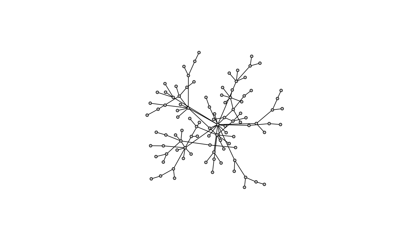

Graphs are initalized with a single node and extended iteratively as new nodes are added to the graph with an edge to an existing node with some probability. This probability is determined partially by the power argument, which gives more or less preference to high-degree nodes. This leads to scale-free structures where a few nodes are hubs in the graph.

g1 <- model.pa(100, power=1)
g2 <- model.pa(100, power=1.3)
g3 <- model.pa(100, power=1.5)

par(mfrow=c(1,3))
model.plot(g1)
model.plot(g2)
model.plot(g3)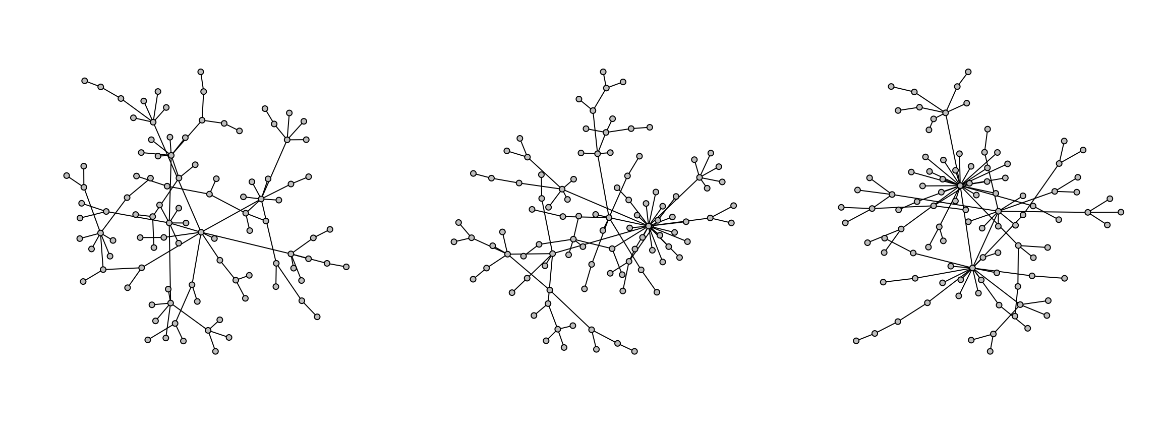

Small World Model

Another relevant model for biological networks utilizes the Watts–Strogatz model for generating random graphs with the small world properties, including short average path lengths and high clustering.

g <- model.sw(100)
model.plot(g)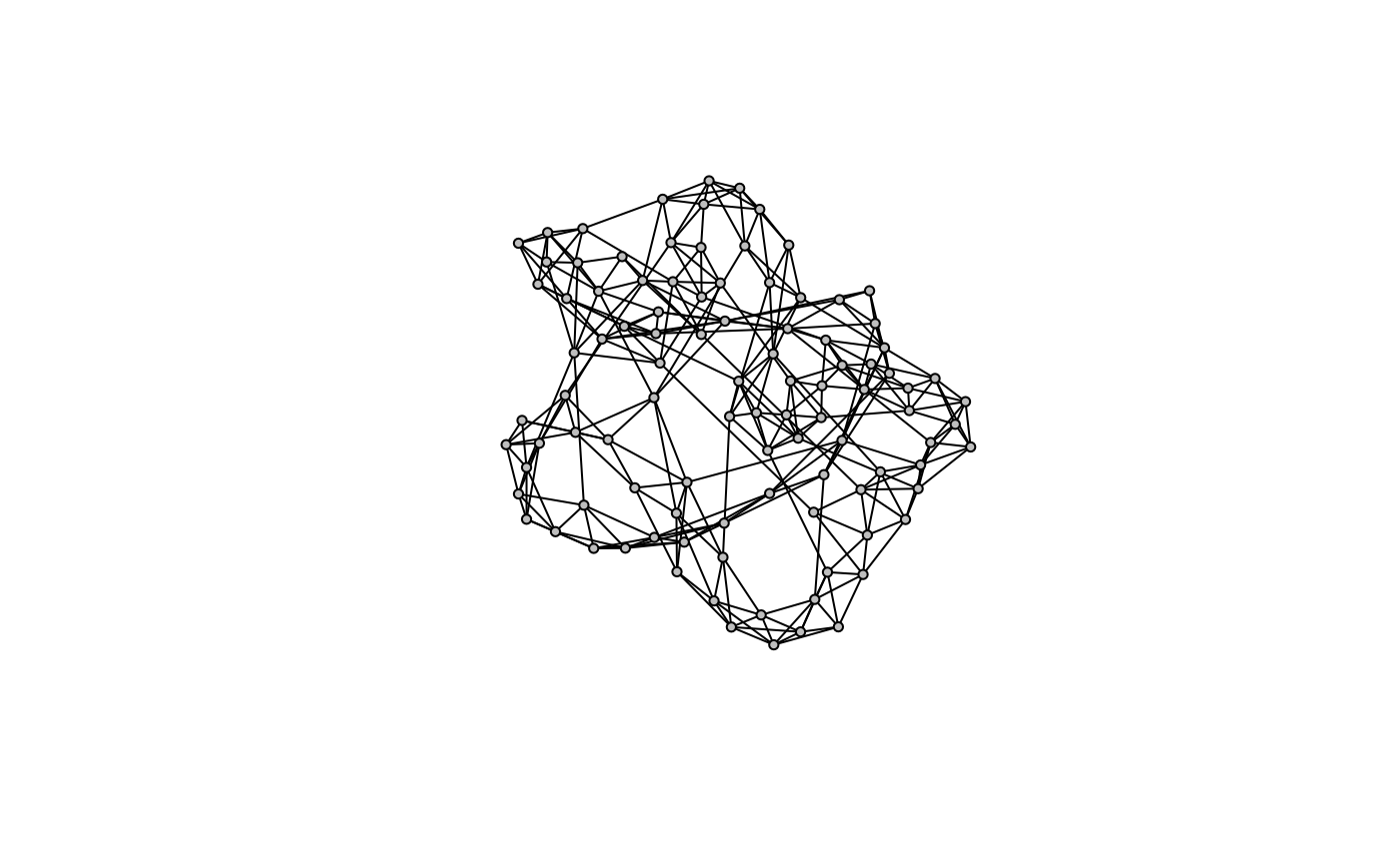

Random Model

Perhaps the simplest model is the Erdős–Rényi model for generating random graphs. Through this algorithm, nodes are initalized and edges are drawn arbitrarily at a given probability.

g <- model.er(100, 0.05)
model.plot(g)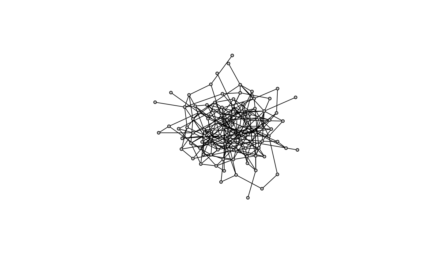

Modular Structures

Modular Preferential Attachment

Here is an extension of the preferential attachment algorithm where multiple scale-free models are randomly connected to simulate networks that have both modular and scale-free properties which are recognized in biological networks.

g <- model.mpa(200)
model.plot(g)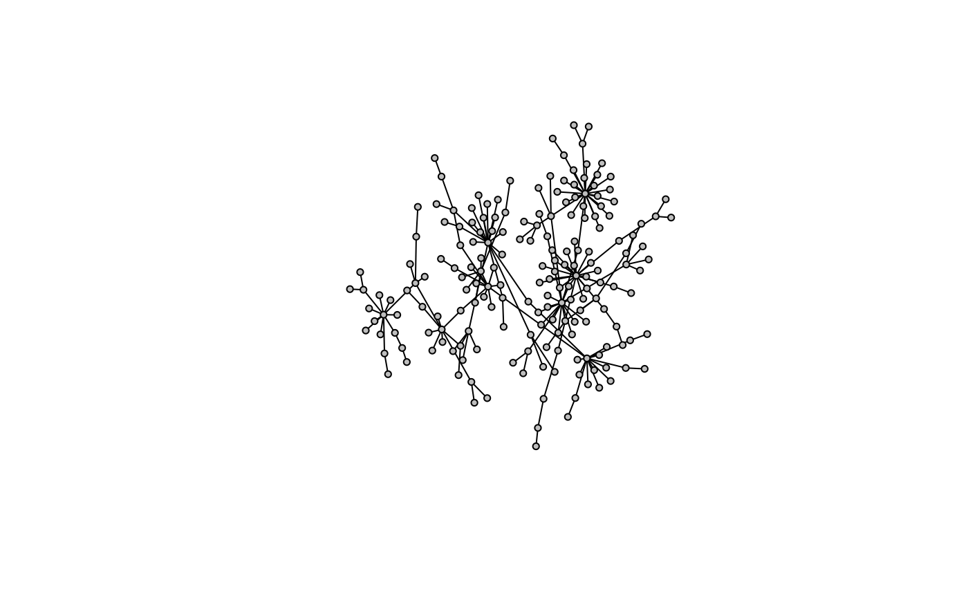

Lancichinetti–Fortunato–Radicchi Benchmark

For a more robust approach to generating modular scale-free networks, we use the LFR model to generate scale-free networks (degree distribution follows a power law) and also contain a modularity component (high clustering coefficient). These are two important structural properties observed in real biological networks. The most robust implementation of LFR is written in python via the networkx package.

This can be installed and used as follows..

pip install networkx
pip install numpy
pip install scipy

import networkx as nx
from networkx.generators.community import LFR_benchmark_graph

G = LFR_benchmark_graph(n=500,
                        tau1=2.7,
                        tau2=2,
                        mu=0.09,
                        max_iters=250,
                        average_degree=5,
                        min_community=10,
                        max_community=50,
                        seed=1,
                        **kwargs)

g <- readRDS(file.path(system.file("extdata", package="shine"), "models.rds"))
model.plot(g)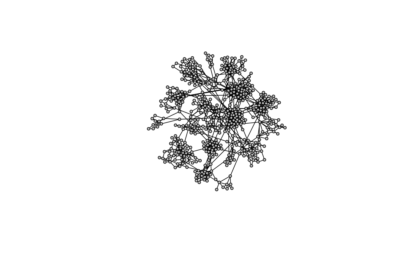

Multiple Networks

When estimating multiple networks underlying similar biological phenotypes, one may assume networks share some structural features. To generate multiple scale-free networks that share features with a known similarity, we can modify the Barabási–Albert algorithm with the following steps:

Seed the algorithm with a relatively small graph
For multiple networks, run the algorithm independently multiple times, each diverging from the seed. Due to the preferential attachment mechanism, hub nodes in one network will remain hubs in another, potentially with different targets.
Calculate the mean pairwise overlap similarity of edges between networks.

g <- model.pa(100, power=1.3)
model.plot(g)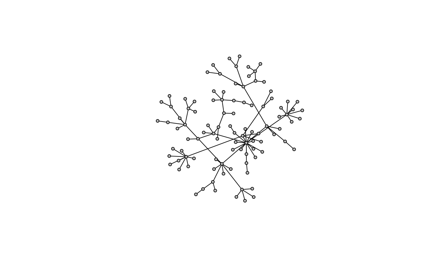

graphs <- model.hpa(3, p=120, seed=g, power=1.3)
models.plot(graphs)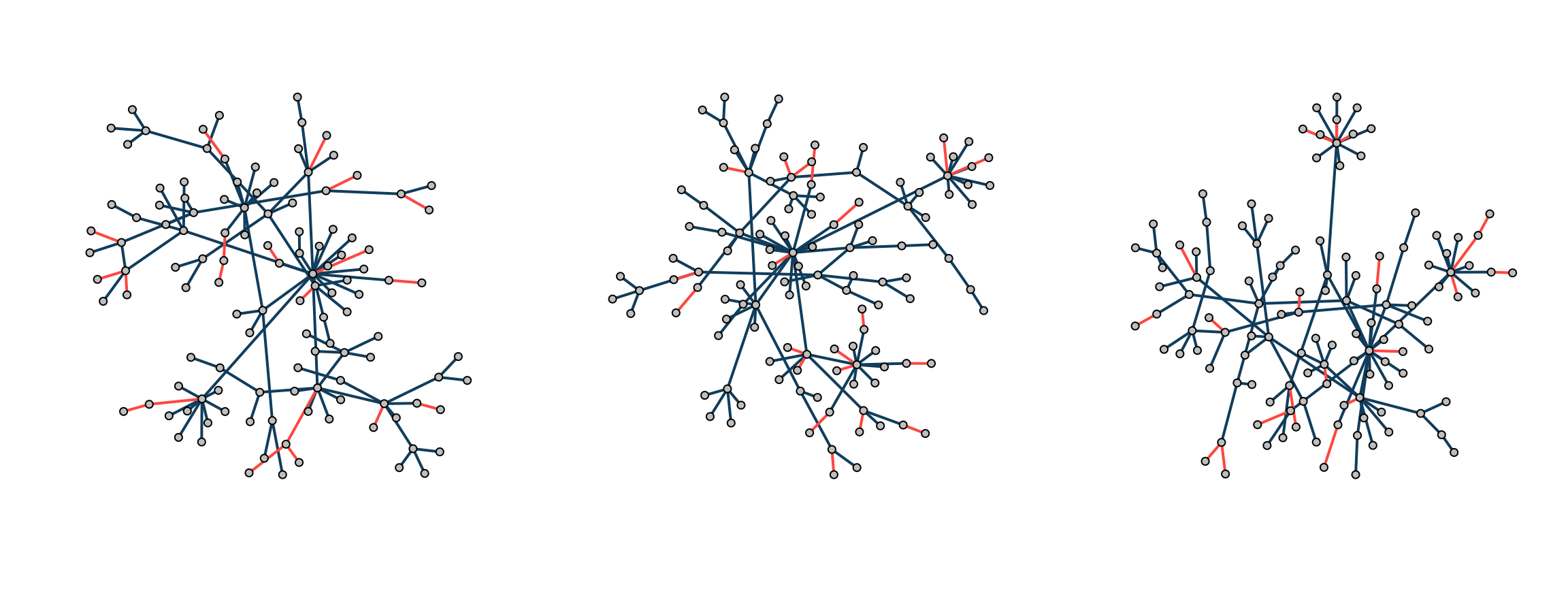

percent(models.similarity(graphs))

[1] "84%"

Generating Data

We can use any of the models to simulate expression data that follows a multivariate Gaussian distribution, which is formatted as an Expression Set object, which is the primary input to downstream functions.

g <- model.pa(100, power=1.3)
data <- model.sim(50, g)
dim(data$eset)

Features  Samples 
     100       50

Network Simulation