Age-Conditioned SHAP Decompositions for Linear Aging Clocks • ClockSHAP

ClockSHAP is an interpretability framework for linear-additive aging clocks (e.g., transcriptomic, epigenetic, or proteomic clocks fit with linear, ridge, or elastic-net regression).

It answers a single question:

Why is this sample predicted to be older or younger than expected for its chronological age?

The method was developed for tissue-of-origin transcriptomic aging clocks but is designed to support comparative aging analyses across diverse clock contexts.

ClockSHAP method overview

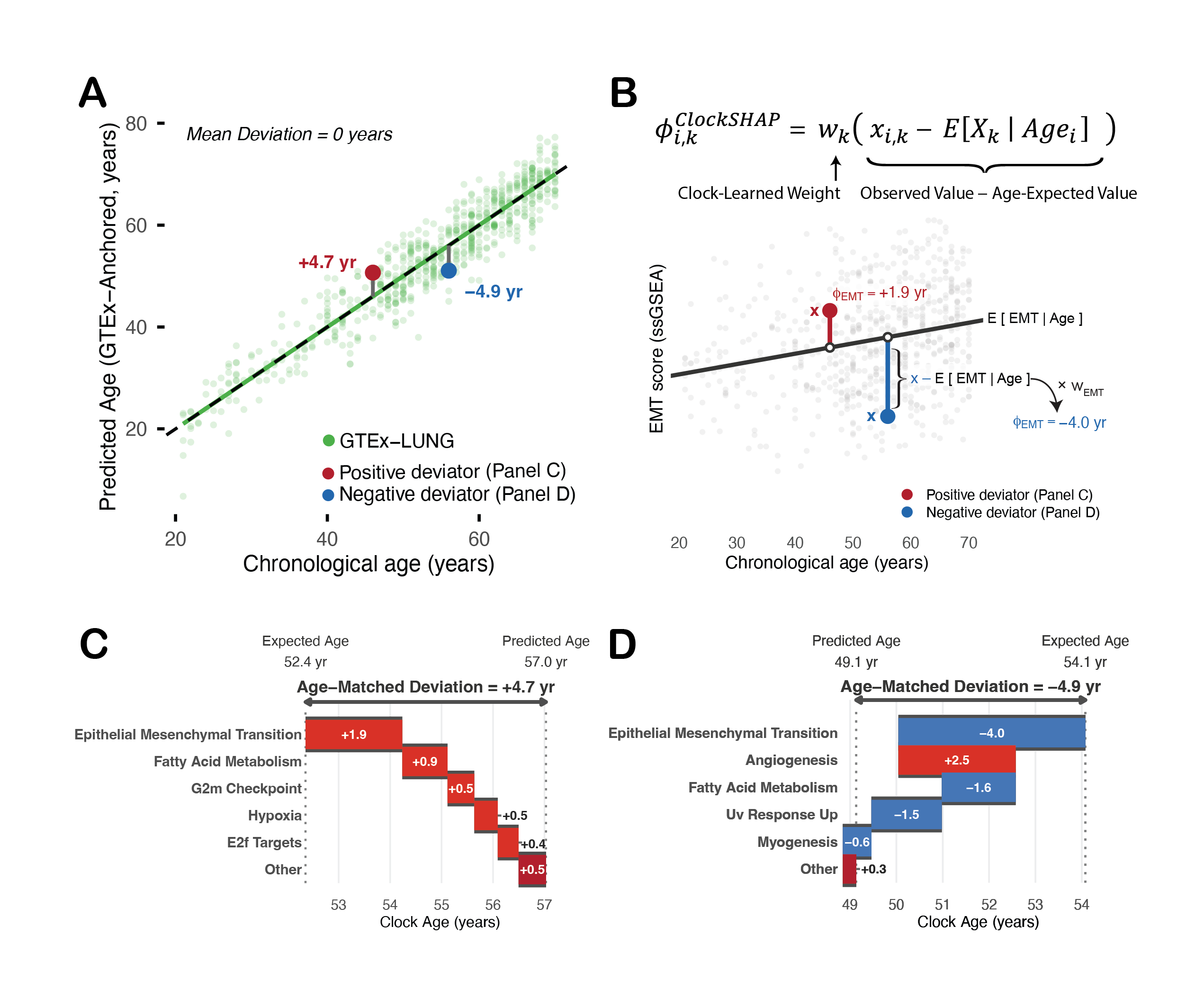
ClockSHAP applied to a lung-tissue aging clock on real GTEx-LUNG data. (A) Predicted vs. chronological age across the cohort, with one positive and one negative deviator highlighted. (B) A single feature’s contribution, computed as its clock weight times its distance from the age-expected value. (C, D) The full per-feature decompositions for the two deviators, with contributions summing exactly to each sample’s age-matched deviation. Figure from [Bock et al., in preparation].

What you get out of ClockSHAP

For each sample, ClockSHAP returns its age-matched deviation (how far the predicted clock age sits above or below what is expected at that chronological age) together with per-feature contributions that sum exactly to that deviation.

The figure above shows this on real lung-tissue data for a pathway-level transcriptomic clock. The positive deviator (Panel C) reads about 4.7 years older than expected, attributed to programs such as epithelial–mesenchymal transition (+1.9 years) and fatty-acid metabolism (+0.9); the negative deviator (Panel D) reads about 4.9 years younger, driven largely by low EMT (−4.0). In both cases the contributions sum exactly to the deviation, a guarantee of the method rather than an approximation.

This output feeds downstream analyses: comparing which features drive deviation across a cohort, deep dives on individual samples, or hypothesis generation about which biological programs are differentially engaged.

Because the reference here is the GTEx-LUNG cohort itself, the deviations shown are exactly the commonly used relative age acceleration (RAA), the residual of predicted age regressed on chronological age, which is why Panel A’s mean deviation is zero. See Terminology: deviation vs. AAA vs. RAA below for the details.

Installation

# Recommended
install.packages("pak")
pak::pak("montilab/ClockSHAP")

# Alternative
install.packages("remotes")
remotes::install_github("montilab/ClockSHAP")

Quick start

ClockSHAP needs three things: a feature matrix (samples in rows, features in columns), a vector of chronological ages (one per sample), and a clock describing how those features map to predicted age. The bundled clockshap_example supplies all three, so we can look at the expected shapes first:

library(ClockSHAP)

# Features: rows are samples, columns are the clock's features.
# (If your matrix is genes x samples, transpose it first.)
clockshap_example$features[1:3, 1:4]
#>        CDKN2A    GDF15    EDA2R      IL6
#> S001 7.034590 7.851806 5.223082 6.046552
#> S002 5.641907 6.397235 5.266366 4.738019
#> S003 5.293459 6.050086 3.950593 4.233756

# One chronological age per sample
head(data.frame(
  sample = names(clockshap_example$age),
  age    = unname(clockshap_example$age)
))
#>   sample  age
#> 1   S001 80.3
#> 2   S002 81.5
#> 3   S003 45.7
#> 4   S004 75.7
#> 5   S005 65.3
#> 6   S006 58.6

# The clock: an intercept (alpha), per-feature weights (beta), and the
# training mean/SD used to standardize each feature (mu, sigma)
str(clockshap_example$clock)
#> List of 4
#>  $ alpha: num 59
#>  $ beta : Named num [1:8] 3.43 3.08 2.65 1.67 -2.08 ...
#>   ..- attr(*, "names")= chr [1:8] "CDKN2A" "GDF15" "EDA2R" "IL6" ...
#>  $ mu   : Named num [1:8] 5.34 6.23 4.46 4.6 5.68 ...
#>   ..- attr(*, "names")= chr [1:8] "CDKN2A" "GDF15" "EDA2R" "IL6" ...
#>  $ sigma: Named num [1:8] 1.034 1.074 0.933 1.126 0.998 ...
#>   ..- attr(*, "names")= chr [1:8] "CDKN2A" "GDF15" "EDA2R" "IL6" ...
#>  - attr(*, "class")= chr "linear_clock"

For your own model you build this object with linear_clock(alpha, beta, mu, sigma) from its fitted coefficients; the feature columns just have to be named to match. With those inputs in hand, the workflow is three calls: fit an age-conditioned reference from the data, run the decomposition, and inspect a sample.

# Age-conditioned reference profile (defines "expected for age"), fit from the data
ref <- fit_reference_profile(
  features = as.data.frame(clockshap_example$features),
  age      = clockshap_example$age
)

# Decompose each sample's age-matched deviation into per-feature contributions
cs <- clockshap(
  features  = clockshap_example$features,
  age       = clockshap_example$age,
  clock     = clockshap_example$clock,
  reference = ref
)

# Inspect one sample's decomposition as a waterfall
plot_clockshap_waterfall(cs, sample = 1, top_n = 6)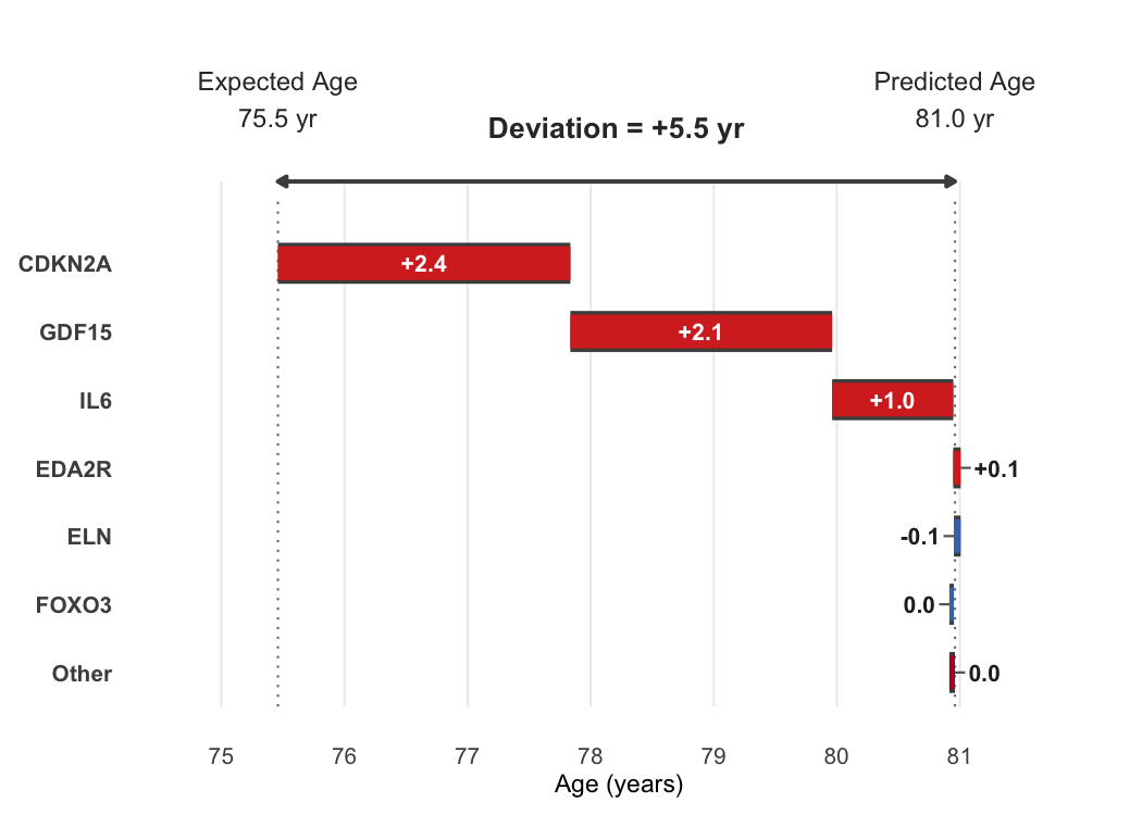

Waterfall decomposition of one synthetic sample's age-matched deviation into per-gene contributions

The returned clockshap object is a list with five fields:

predicted: clock prediction $\hat{y}$
expected: age-matched expectation $\mathrm{E}[\hat{y} \mid \mathrm{Age}]$ under the reference
deviation: predicted - expected ( $\Delta$ )
phi: per-feature contribution matrix (rows sum exactly to deviation)
age: input chronological ages

For a complete worked example, including the cohort scatter, per-sample waterfalls, and comparison with age-acceleration metrics, read the ClockSHAP introduction vignette. The documentation site also includes the full function reference.

How it works (in two lines)

ClockSHAP is built around two identities. The first defines what it explains: the age-matched deviation of a sample’s predicted age from its age-matched expectation,

$\Delta_i = \hat{y}_i - \mathrm{E}[\hat{y} \mid \mathrm{Age}_i]$

The second is the exact additive decomposition of that deviation into per-feature contributions,

$\sum_k \phi_{i,k} = \Delta_i$

Here $\hat{y}$ is the clock’s predicted age, $\mathrm{E}[\hat{y} \mid \mathrm{Age}]$ is the age-matched expectation under a reference, and $\phi$ is a single feature’s contribution. Everything below is about how the expectation and the contributions are defined, and why the decomposition is exact.

The building blocks

The rest of this README explains the two identities above:

what expected means (the reference profile),
why the per-feature contributions $\phi_k$ sum exactly to the deviation (the SHAP property),
how the deviation differs from other clock-acceleration metrics (AAA, RAA).

How `expected` is defined: the reference profile

Aging-clock features change systematically with chronological age, so a single global baseline is inappropriate for comparing samples of different ages. ClockSHAP instead uses an age-conditioned reference. For each feature $k$ it fits an age trend on a reference cohort:

$\mathrm{E}[X_k \mid \mathrm{Age}] = \gamma_{0,k} + \gamma_{1,k}\,\mathrm{Age}$

Passing this age-expected feature vector through the clock $f$ gives the age-matched expectation, and the deviation is the gap from it:

$\mathrm{E}[\hat{y} \mid \mathrm{Age}] = f\big(\mathrm{E}[X \mid \mathrm{Age}]\big), \qquad \Delta = \hat{y} - \mathrm{E}[\hat{y} \mid \mathrm{Age}]$

So expected is the clock’s typical output for reference individuals of the same chronological age, and the deviation is how far above or below that a sample lies.

Reference note. Because expected depends on the chosen reference (e.g., GTEx tissue-of-origin), the deviation should be interpreted relative to that reference; it is not a universal biological-age score.

Interpretation note. The deviation is a cross-sectional state shift relative to an age-matched expectation; it does not by itself imply a within-individual aging rate.

Why the contributions sum exactly to the deviation: the SHAP property

For linear-additive models, SHAP-style attributions have a closed form. ClockSHAP’s per-feature contribution is the feature’s clock weight $w_k$ times its distance from the age-expected value, the form shown in Panel B of the figure above:

$\phi_{i,k} = w_k\big(x_{i,k} - \mathrm{E}[X_k \mid \mathrm{Age}_i]\big)$

Summed over features, the contributions recover the deviation exactly:

$\sum_k \phi_{i,k} = \Delta_i$

Implementation note. In practice the features are standardized to the clock’s training distribution (mean and standard deviation) before the decomposition is computed. Changing the reference changes the expectation, and therefore the decomposition target, so every component is reference-anchored.

Terminology: deviation vs. AAA vs. RAA

ClockSHAP explains $\Delta = \text{predicted} - \text{expected}$ , not raw prediction error. Two other quantities appear in the aging-clock literature:

Absolute age acceleration (AAA, sometimes called ΔAge):

$\mathrm{AAA} = \hat{y} - \mathrm{Age}$

Simple, but age-biased when the clock slope is below 1: younger samples are over-predicted and older samples under-predicted.

Relative age acceleration (RAA, regression residuals):

RAA <- residuals(stats::lm(predicted ~ age))

A post-hoc calibration that removes systematic age trends in prediction error within a chosen cohort.

ClockSHAP deviation. ClockSHAP’s $\Delta$ generalizes RAA. The age-conditional expectation is built through a feature-level reference profile ( $\gamma_0 + \gamma_1\,\mathrm{Age}$ per feature, passed through the clock) rather than by regressing $\hat{y}$ on age directly. This has an exact special case: for a linear-additive clock, when the reference is fit on the cohort of interest itself, $\Delta$ equals RAA sample-for-sample. Because $\hat{y}$ is an exact linear function of the features and OLS projection onto age is linear, passing the per-feature age trends through the clock reproduces the OLS fit of $\hat{y} \sim \mathrm{Age}$ exactly, so $\text{predicted} - \text{expected} = \text{predicted} - \text{fitted} = \text{residual} = \mathrm{RAA}$ .

An additional usage of ClockSHAP is what happens when the reference is set to a different, biologically meaningful cohort (e.g., GTEx tissue-of-origin): expected is then anchored to normal aging in that reference rather than to the target cohort’s own internal trend, and the deviation measures departure from that external expectation.

We recommend the name “deviation” or “age-matched deviation” to keep this distinct from AAA and RAA.

Practical notes

Deviation is reference-dependent. The choice of reference cohort defines what “expected for age” means.
“Years” are clock-relative. A deviation of +5 under one clock is not comparable to +5 under a different clock, training set, or feature space.
Upstream preprocessing matters a lot. ClockSHAP assumes the feature matrix is analysis-ready and consistent with the clock (transformations, normalization, feature matching, batch correction, QC). Mismatched feature spaces or batch effects produce technical, not biological, deviations. The importance of this step cannot be overstated.

For broader discussion of calibration, age bias, and computational challenges in clock analysis, see Epigenetic ageing clocks: statistical methods and emerging computational challenges (Nature Reviews Genetics).

Status

Under active development.

ClockSHAP