Introduction to ClockSHAP

Overview

ClockSHAP interprets the output of a linear aging clock. Instead of asking which features push a predicted age up or down in absolute terms, it answers:

Why is this sample predicted to be older or younger than expected for its chronological age?

For a linear clock it provides an exact, closed-form decomposition of that gap into per-feature contributions. This vignette walks through the full workflow on the package’s bundled synthetic dataset: the data, the core objects, the decomposition, the accessors, and how the result relates to the more familiar age-acceleration metrics.

The method in brief

A linear clock predicts age, $\hat{y}$, from features. ClockSHAP defines the age-matched deviation as the gap between that prediction and the age-matched expectation under a reference:

$$\Delta_i = \hat{y}_i - \mathrm{E}[\hat{y} \mid \mathrm{Age}_i]$$

The expectation comes from an age-conditioned reference profile, a per-feature linear age trend fit on a reference cohort:

$$\mathrm{E}[X_k \mid \mathrm{Age}] = \gamma_{0,k} + \gamma_{1,k}\,\mathrm{Age}$$

Each feature’s contribution is its clock weight $w_k$ times its distance from that age-expected value, and for a linear clock the contributions reconstruct the deviation exactly:

$$\phi_{i,k} = w_k\big(x_{i,k} - \mathrm{E}[X_k \mid \mathrm{Age}_i]\big), \qquad \sum_k \phi_{i,k} = \Delta_i$$

In practice features are standardized to the clock’s training distribution before the decomposition is computed.

The example data

The package ships a small, fully synthetic dataset, clockshap_example, so every example runs without external data. It is a list with three pieces:

str(clockshap_example, max.level = 1)
#> List of 3
#>  $ features: num [1:120, 1:8] 7.03 5.64 5.29 7.15 5.03 ...
#>   ..- attr(*, "dimnames")=List of 2
#>  $ age     : Named num [1:120] 80.3 81.5 45.7 75.7 65.3 58.6 70.5 37.4 66.1 68.8 ...
#>   ..- attr(*, "names")= chr [1:120] "S001" "S002" "S003" "S004" ...
#>  $ clock   :List of 4
#>   ..- attr(*, "class")= chr "linear_clock"

features is a 120 × 8 matrix of synthetic “gene” values (rows S001–S120), each gene carrying a genuine linear age trend plus noise; age is the chronological age; and clock is a fitted clock object. Note the layout: rows are samples and columns are the clock’s features, so transpose a genes × samples matrix first. Two samples are planted deviators: S001 reads older than expected for its age and S002 reads younger, both driven by a shared senescence / inflammaging axis (CDKN2A, GDF15, IL6). The data carry no real biological signal; the gene symbols are only there to make the output legible.

The building blocks: clock and reference

ClockSHAP works with two specification objects.

A linear_clock holds the intercept, the per-feature weights, and the training mean and standard deviation used to standardize features. You construct one with linear_clock(); here we inspect the bundled clock:

clock <- clockshap_example$clock
class(clock)
#> [1] "linear_clock"
round(clock$beta, 2)   # per-gene weights learned by the clock
#> CDKN2A  GDF15  EDA2R    IL6  LMNB1    ELN COL1A1  FOXO3 
#>   3.43   3.08   2.65   1.67  -2.08  -2.49   2.61  -2.30

A reference_profile holds, for each feature, the intercept and slope of its age trend ($\gamma_0$, $\gamma_1$). You can build one directly with reference_profile(gamma0, gamma1), but usually you fit it from a cohort with fit_reference_profile(), which regresses each feature on age:

ref <- fit_reference_profile(
  features = as.data.frame(clockshap_example$features),
  age      = clockshap_example$age
)
class(ref)
#> [1] "reference_profile"
round(ref$gamma1, 4)   # per-gene age slopes recovered from the cohort
#>  CDKN2A   GDF15   EDA2R     IL6   LMNB1     ELN  COL1A1   FOXO3 
#>  0.0459  0.0412  0.0354  0.0364 -0.0357 -0.0393  0.0359 -0.0417

The non-zero slopes confirm the features genuinely move with age, which is what makes the age-conditioned expectation meaningful.

Running ClockSHAP

clockshap() ties the pieces together: features, ages, a clock, and a reference. It standardizes the features with the clock’s parameters, builds the age-matched expectation from the reference, and returns the decomposition.

cs <- clockshap(
  features  = clockshap_example$features,
  age       = clockshap_example$age,
  clock     = clockshap_example$clock,
  reference = ref
)

cs                # print method: dimensions + deviation range
#> <ClockSHAP object>
#>   Samples : 120 
#>   Features: 8 
#> 
#>   Deviation range:
#>     Min: -12.921 
#>     Max: 12.982
summary(cs)$deviation
#>     Min.  1st Qu.   Median     Mean  3rd Qu.     Max. 
#> -12.9211  -3.5435   0.4285   0.0000   4.0046  12.9823

clockshap() also enforces its core invariant internally: it will error rather than return a result where the contributions fail to sum to the deviation.

The output: structure and accessors

A clockshap object is a list with five elements, each retrievable either by $ or with an accessor function:

field	accessor	meaning
predicted	clockshap_predicted()	clock prediction $\hat{y}$
expected	clockshap_expected()	age-matched expectation $\mathrm{E}[\hat{y}\mid\mathrm{Age}]$
deviation	clockshap_deviation()	$\Delta = \text{predicted} - \text{expected}$
phi	clockshap_phi()	per-feature contribution matrix (samples × features)
age	(none)	the input chronological ages

head(data.frame(
  age       = cs$age,
  predicted = round(clockshap_predicted(cs), 1),
  expected  = round(clockshap_expected(cs), 1),
  deviation = round(clockshap_deviation(cs), 1)
))
#>       age predicted expected deviation
#> S001 80.3      81.0     75.5       5.5
#> S002 81.5      70.8     76.4      -5.6
#> S003 45.7      47.9     48.8      -0.9
#> S004 75.7      70.5     71.9      -1.4
#> S005 65.3      55.7     63.9      -8.2
#> S006 58.6      59.3     58.7       0.6

The contributions in clockshap_phi() sum, row by row, exactly to the deviation:

all.equal(rowSums(clockshap_phi(cs)), clockshap_deviation(cs), tolerance = 1e-10)
#> [1] "names for target but not for current"

Cohort view

Plotting each sample’s predicted age against its chronological age reproduces the cohort-level picture. The black line is the age-matched expectation; a sample’s vertical distance from it is its deviation. The two planted deviators sit clearly off the line.

library(ggplot2)

cohort <- data.frame(
  age       = cs$age,
  predicted = clockshap_predicted(cs),
  role      = ifelse(rownames(clockshap_example$features) == "S001", "S001 (older)",
               ifelse(rownames(clockshap_example$features) == "S002", "S002 (younger)",
                      "cohort"))
)

ggplot(cohort, aes(age, predicted)) +
  geom_point(data = subset(cohort, role == "cohort"),
             colour = "grey70", alpha = 0.7) +
  geom_smooth(method = "lm", se = FALSE, colour = "black", linewidth = 0.6) +
  geom_point(data = subset(cohort, role != "cohort"),
             aes(colour = role), size = 3) +
  scale_colour_manual(values = c("S001 (older)" = "#B2182B",
                                 "S002 (younger)" = "#2166AC")) +
  labs(x = "Chronological age (years)", y = "Predicted age (years)", colour = NULL) +
  theme_minimal()
#> `geom_smooth()` using formula = 'y ~ x'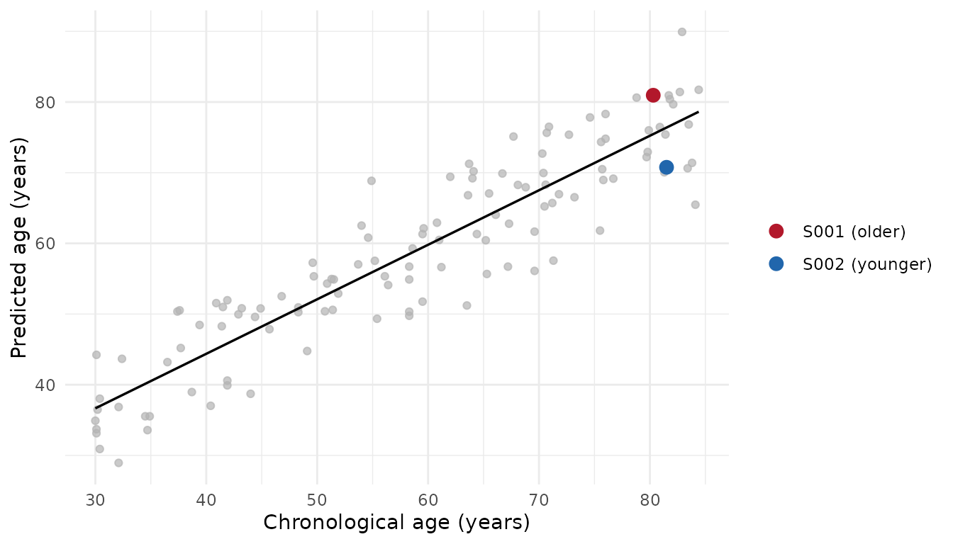

Age-matched deviation vs. AAA and RAA

It helps to see how the deviation relates to two metrics common in the aging-clock literature:

• Absolute age acceleration (AAA): $\hat{y} - \mathrm{Age}$.
• Relative age acceleration (RAA): the residuals of lm(predicted ~ age).

age  <- cs$age
pred <- clockshap_predicted(cs)

metrics <- data.frame(
  AAA       = pred - age,
  RAA       = as.numeric(residuals(lm(pred ~ age))),
  deviation = clockshap_deviation(cs)
)

Because this clock has a slope below 1, AAA is age-biased, systematically positive for younger samples and negative for older ones, while RAA and the deviation are not:

round(sapply(metrics, function(z) cor(z, age)), 3)
#>       AAA       RAA deviation 
#>    -0.565     0.000     0.000

And here the reference was fit on the same cohort we are analyzing. In that self-reference case the age-matched deviation is exactly relative age acceleration:

all.equal(metrics$deviation, metrics$RAA, tolerance = 1e-9)
#> [1] TRUE

This is not a coincidence: for a linear clock, passing per-feature age trends through the clock reproduces the OLS fit of predicted age on age, so predicted - expected equals the regression residual. ClockSHAP becomes distinct from RAA, and starts carrying new biological signal, only when the reference is a different, biologically meaningful cohort (e.g., a tissue-of-origin reference). What it always adds, even in the self-reference case, is the per-feature attribution of that deviation, which neither AAA nor RAA provides.

Per-sample decomposition

plot_clockshap_waterfall() shows, for a single sample, how each feature carries the prediction from the age-matched expectation to the predicted age. The bars sum to the deviation. Compare the two planted deviators:

plot_clockshap_waterfall(cs, sample = "S001", top_n = 6)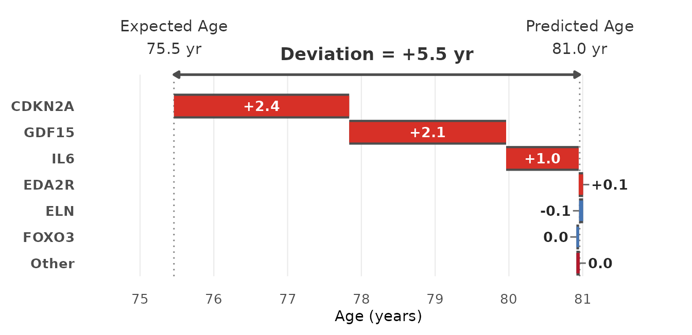

plot_clockshap_waterfall(cs, sample = "S002", top_n = 6)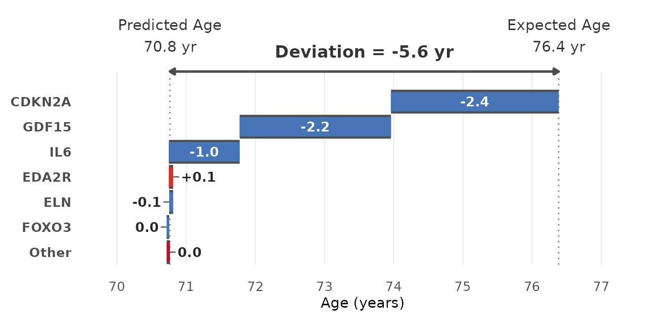

S001 reads older because its senescence / inflammaging genes sit above their age-expected levels; S002 reads younger for the mirror-image reason. In both, the labeled contributions add up to the age-matched deviation.

Scope and assumptions

ClockSHAP is defined for linear aging clocks and requires:

• linear, additive feature contributions (a linear_clock),
• an age–feature reference relationship (a reference_profile),
• consistent feature definitions between the clock and the reference.

It does not train clocks, and it does not assume a particular source of reference data; any cohort can define the reference aging trajectory. Because the choice of reference determines what “expected for age” means, deviations should always be interpreted relative to it.