CaDrA.shiny

---

An R Shiny Dashboard for Interacting with CaDrA Package

CaDrA Package: https://montilab.github.io/CaDrA/

Web Portal: https://cadra.bu.edu/

Overview

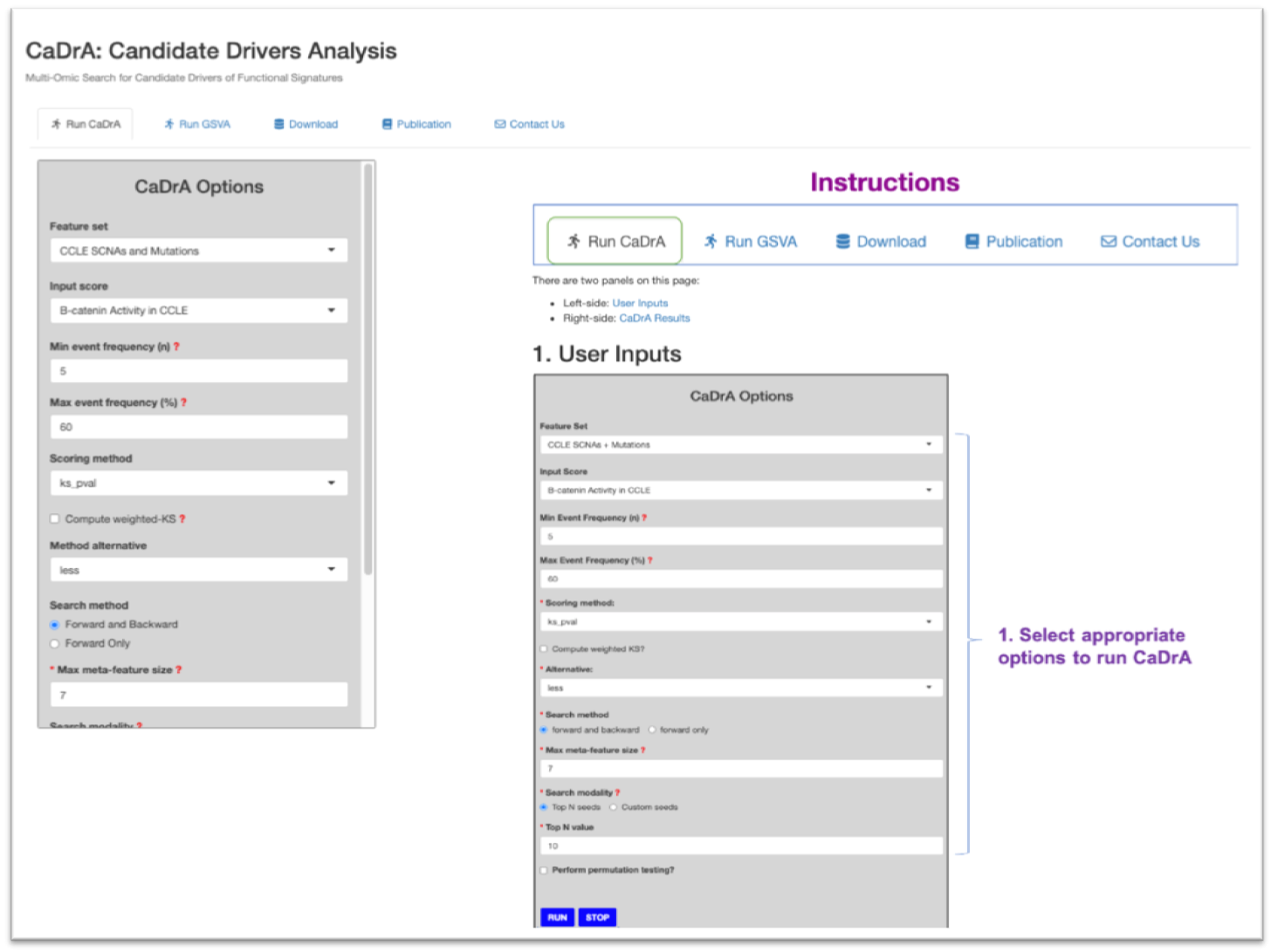
CaDrA.shiny is an interactive R Shiny dashboard developed to allow users to directly interact with CaDrA package. CaDrA is an R package that supports a heuristic search framework aimed at identifying candidate drivers of a molecular phenotype of interest (visit our Github repo for more details).

The CaDrA’s Shiny dashboard has two distinctive features:

1. Run CaDrA search to identify candidate drivers of a molecular phenotype of interest.
2. Run GSVA to estimate aggregate enrichment scores by projecting a (gene) expression dataset onto a given gene set or signature, usually representing a molecular phenotype. Afterward, one can apply CaDrA search to look for genetic drivers based on a given binary multi-omics dataset and its derived enrichment score of a signature of interest.

Data visualizations include:

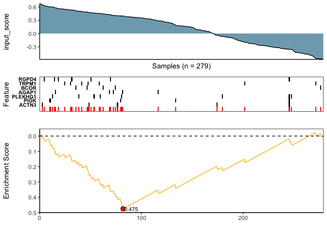
• Meta-feature plot.
• Kolmogorov Smirnov (KS) enrichment plot.
• Top N candidates overlapping heatmap.
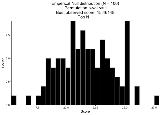
• Permutation plot.

CaDrA.shiny is currently containerized using Docker and can be deployed on any compatible cloud-based services.

Docker image: montilab/cadra-shiny

Useful Guides

• Launch CaDrA’s Shiny Dashboard with Docker
• Launch CaDrA’s Shiny Dashboard with Compose

(1) Installation

# Install BiocManager
if (!require("BiocManager", quietly = TRUE))
  install.packages("BiocManager")

# Install CaDrA 
BiocManager::install("CaDrA")

# Install GSVA 
BiocManager::install("GSVA")

# Install hypeR
library(devtools)
devtools::install_github("montilab/hypeR")

# Install CaDrA.shiny
devtools::install_github("montilab/CaDrA.shiny")

(2) Load packages

library(CaDrA.shiny)
library(CaDrA)
library(GSVA)
library(hypeR)

(3) Run CaDrA with dataset downloaded from CaDrA Portal

Here, we show how to run CaDrA on a dataset downloaded from the CaDrA Portal, using input_score’s derived by applying GSVA to the downloaded gene expression dataset and the Hallmarks genesets. We will run a CaDrA search to look for genetic drivers of the “Epithelial Mesenchymal Transition” (EMT)-derived score.

(i) Retrieve a list of descriptors of pre-processed feature sets available on the portal

## Get a list of descriptors of feature sets available on CaDrA Portal
fs_list <- CaDrA.shiny::get_feature_set(order_by="asc")

## Show the description of the first few feature sets
knitr::kable(head(fs_list), row.names = FALSE)

feature_set_name	description	collection
CCLE SCNAs and Mutations	Somatic copy number alterations and mutations from CCLE. See ?CaDrA::CCLE_MUT_SCNA	CCLE
Simulated Feature Set	Simulated feature set comprises of 1000 genomic features and 100 sample profiles. This simulated data includes 10 left-skewed (i.e. True Positive or TP) and 990 uniformly-distributed (i.e. True Null or TN) features. See ?CaDrA::BRCA_GISTIC_MUT_SIG	Simulated
TCGA BrCa SCNAs and Mutations	Somatic copy number alterations and mutations from BRCA TCGA. See ?CaDrA::BRCA_GISTIC_MUT_SIG	TCGA
TCGA_ACC_2016_01_28_GISTIC_MUT_SIG	ACC	TCGA
TCGA_BLCA_2016_01_28_GISTIC_MUT_SIG	BLCA	TCGA
TCGA_BRCA_2016_01_28_GISTIC_MUT_SIG	BRCA	TCGA

(ii) Retrieve datasets from the portal

## Retrieve the dataset (both genetic feature set and gene expression)
datasets <- CaDrA.shiny::pull_datasets(
  feature_set = "TCGA_HNSC_2016_01_28_GISTIC_MUT_SIG",
  include_gene_expression = TRUE
)
datasets

$feature_set
class: RangedSummarizedExperiment 
dim: 12852 279 
metadata(3): experimentData annotation protocolData
assays(1): exprs
rownames(12852): Amp2q11.2 Amp2q31.2 ... ZZEF1 ZZZ3
rowData names(1): Feature
colnames(279): TCGA-BA-4074-01 TCGA-BA-4076-01 ... TCGA-IQ-7631-01
  TCGA-IQ-7632-01
colData names(0):

$gene_expression
class: RangedSummarizedExperiment 
dim: 20234 566 
metadata(3): experimentData annotation protocolData
assays(1): exprs
rownames(20234): SMR3B STATH ... SCARNA27 MS4A5
rowData names(1): Genes
colnames(566): TCGA-4P-AA8J-01 TCGA-BA-4074-01 ... TCGA-WA-A7GZ-01
  TCGA-WA-A7H4-01
colData names(1): Samples

(iii) Run GSVA on the downloaded expression dataset

## download MSigDB’s Hallmark genesets
hallmarks <- hypeR::msigdb_gsets("Homo sapiens", "H", clean=TRUE)$genesets # returns 50 genesets 

# Compute the gsva scores of the 50 hallmark genesets
input_score_matrix <- GSVA::gsva(
  expr = SummarizedExperiment::assay(datasets$gene_expression), 
  gset.idx.list = hallmarks,
  method = "gsva",
  mx.diff = TRUE,
  verbose = FALSE
)

## Show few entries of the returned hallmark-by-sample matrix
knitr::kable(input_score_matrix[1:5, 1:5])

	TCGA-4P-AA8J-01	TCGA-BA-4074-01	TCGA-BA-4075-01	TCGA-BA-4076-01	TCGA-BA-4077-01
Adipogenesis	-0.0160921	0.1648353	0.2211107	-0.0737085	-0.0115116
Allograft Rejection	-0.0049091	-0.0081298	-0.0447976	-0.3880485	0.4610353
Androgen Response	-0.3956958	0.0941687	0.1397883	0.1266452	0.2823991
Angiogenesis	0.3141972	0.2880628	0.3441984	-0.1819343	0.0226343
Apical Junction	0.1902571	-0.2399212	-0.1048696	-0.0193586	0.1687033

(iv) Run candidate search with input scores obtained in (iii)

## Samples to keep based on the overlap between the two inputs
sample_overlap <- intersect(colnames(input_score_matrix), colnames(datasets$feature_set))
input_score <- input_score_matrix["Epithelial Mesenchymal Transition", sample_overlap]
FS <- datasets$feature_set[, sample_overlap, drop = FALSE]

## Pre-filter FS based on occurrence frequency
FS_filtered <- CaDrA::prefilter_data(
  FS = FS,
  max_cutoff = 0.6,  # max event frequency (60%)
  min_cutoff = round(5/ncol(FS), 2)  # make sure min event frequency has at least 5 samples 
)  

## Run candidate search
topn_result <- CaDrA::candidate_search(
  FS = FS_filtered,
  input_score = input_score,
  method = "ks_pval",          # Use Kolmogorov-Smirnov scoring function 
  method_alternative = "less", # Use one-sided hypothesis testing
  weights = NULL,              # If weights are provided, perform a weighted-KS (gsea-like) test
  search_method = "both",      # Apply both forward and backward search
  top_N = 1,                   # Perform only one search (starting from top scoring feature)
  max_size = 7,                # Maximum number of features to include in the returned meta-feature
  do_plot = FALSE,             # Plot after finding the best features
  best_score_only = FALSE      # Return all results from the search
)

(v) Visualize Best Results

## Fetch the meta-feature yielding the best score over N searches
## .. (in this example, only N=1 search was performed)
topn_best_meta <- CaDrA::topn_best(topn_result)

## Visualize the best results with the meta-feature plot
CaDrA::meta_plot(topn_best_list = topn_best_meta, input_score_label = NULL)

(vi) Compute permutation-based p-value

## Permutation seed (for reproducible results)
set.seed(123)

## Run CaDrA Search 100 times on permuted input scores to estimate the null distribution
perm_res <- CaDrA::CaDrA(
  FS = FS_filtered, 
  input_score = input_score, 
  method = "ks_pval",
  method_alternative = "less",
  top_N = 1,
  max_size = 7,
  search_method = "both",     
  n_perm = 100,
  perm_alternative = "one.sided",
  ncores = 2,
  cache = FALSE
)

## Visualize permutation results
CaDrA::permutation_plot(perm_res = perm_res)

(4) Launch CaDrA’s Shiny dashboard with your pre-proccessed dataset

Here, we show how to launch a local instance of the CaDrA Portal, which will be populated with a user-selected set of datasets. In the example, a single dataset (ACC) will be uploaded to the portal.

(i) Pull pre-processed feature sets using our REST API

# Download feature sets from CaDrA portal and return a datalist with appropriate paths to dataset
mydatafile <- CaDrA.shiny::download_feature_sets(
  #feature_set = fs_list$feature_set_name,  # this would download all TCGA datasets
  feature_set = "TCGA_ACC_2016_01_28_GISTIC_MUT_SIG",
  include_input_score = TRUE,
  include_gene_expression = TRUE,
  out_dir = file.path(Sys.getenv("HOME"), "Github") # specify your folder of choice here
)

# Look at the top 6 rows
knitr::kable(head(mydatafile), row.names = FALSE)

feature_set_name	feature_set_path	input_score_name	input_score_path	gene_expression_name	gene_expression_path
TCGA_ACC_2016_01_28_GISTIC_MUT_SIG	/Users/reinachau/Github/download-fs-2023-11-27/TCGA_ACC_2016_01_28_GISTIC_MUT_SIG/feature_set/TCGA_ACC_2016_01_28_GISTIC_MUT_SIG.rds	NA	/Users/reinachau/Github/download-fs-2023-11-27/TCGA_ACC_2016_01_28_GISTIC_MUT_SIG/input_score/NA	TCGA_ACC_2016_01_28_Gene_Expression	/Users/reinachau/Github/download-fs-2023-11-27/TCGA_ACC_2016_01_28_GISTIC_MUT_SIG/gene_expression/TCGA_ACC_2016_01_28_Gene_Expression.rds
TCGA_ACC_2016_01_28_GISTIC_MUT_SIG	/Users/reinachau/Github/download-fs-2023-11-27/TCGA_ACC_2016_01_28_GISTIC_MUT_SIG/feature_set/TCGA_ACC_2016_01_28_GISTIC_MUT_SIG.rds	NA	/Users/reinachau/Github/download-fs-2023-11-27/TCGA_ACC_2016_01_28_GISTIC_MUT_SIG/input_score/NA	TCGA_ACC_2016_01_28_Gene_Expression	/Users/reinachau/Github/download-fs-2023-11-27/TCGA_ACC_2016_01_28_GISTIC_MUT_SIG/gene_expression/TCGA_ACC_2016_01_28_Gene_Expression.rds

(iii) Launch Shiny dashboard with downloaded dataset

## Launch CaDrA's Shiny app with your downloaded datalist retrieved from (ii)
app <- CaDrA.shiny::CaDrA_App(id="myapp", datalist=mydatafile)

## Launch app on localhost with port 3838
shiny::runApp(app, host='0.0.0.0', port=3838)

A Glimpse of CaDrA’s Shiny Dashboard

There are five tabs on CaDrA’s Shiny dashboard. Explore each tab and see what they do.

• Run CaDrA
• Run GSVA
• Download
• Publication
• Contract Us

Getting Help

To get help with CaDrA, visit our Github CaDrA dicussion or Github CaDrA issues.

To get help with CaDrA.shiny, visit our Github CaDrA.shiny dicussion or Github CaDrA.shiny issues.