Publication Annotations • ppi.context

Requirements

library(magrittr)
library(dplyr)
library(ggplot2)
library(ggpubr)
library(igraph)

Data

As a supporting dataset, we have generated information regarding how many PPIs a given publication (pid) is responsible for as well as the number of cell line annotations that were extracted from the text - which allows users to better assess the specificity of PPIs mapped to cell lines.

publications <- read.delim("data/v_1_00/Publications.txt")

Here you can see five cell lines were extracted from publication 28514442 while only a single cell line was extracted from publication 25416956.

head(publications)

       pid n_ppi                            cell_names n_annotations
1 28514442 56297 MCF-10A,HEK293T,HeLa,HCT 116,MCF-10AT             5
2 26186194 23663          HEK293T,HeLa,SH-SY5Y,HeLa S3             4
3 26344197 16625       HeLa,Schneider 2,HCT 116,HEK293             4
4 26496610 15458                            HeLa Kyoto             1
5 25416956 14233                                   HEK             1
6 22939629 13912                   HeLa,HEK293,HeLa S3             3
  specificity
1         5-9
2         2-4
3         2-4
4           1
5           1
6         2-4

Interactions reported per publication

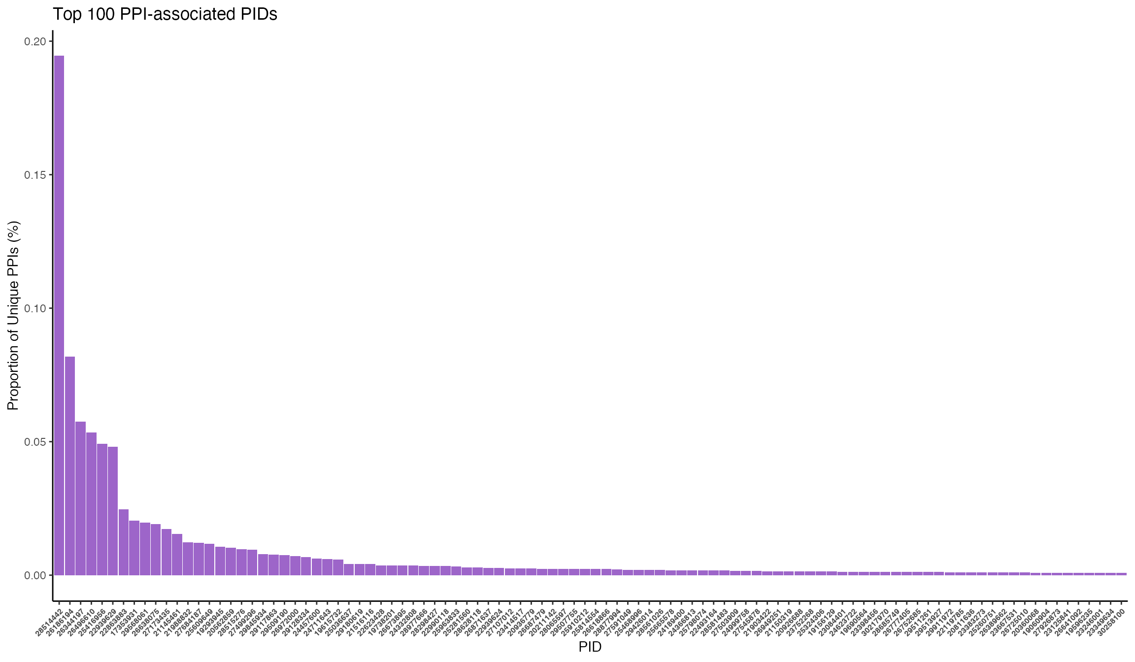
It is important to note that a large percentage of the interactions come from a single study. Here they present BioPlex 2.0, a high-throughpout method for expression and purification for proteins in HEK293T cells and employs robust affinity purification-mass spectrometry (AP-MS) to the interrogation of protein-protein interactions. They report 56297 unique PPIs. Users may want to filter out these PPIs if they want to remove non-specific PPIs purified from cell lines primarily used as efficient expression vectors such as HEK.

publication.info(28514442)

PMID: 28514442
Huttlin EL et. al. (2017) Nature
Architecture of the human interactome defines protein communities and disease networks.

publications %>%
dplyr::mutate(ppi_pct = n_ppi / sum(n_ppi)) %>%
dplyr::arrange(desc(ppi_pct)) %>%
dplyr::mutate(pid = factor(pid, levels=pid)) %>%
head(100) %>%
ggplot(aes(x=pid, y=ppi_pct)) +
geom_bar(stat="identity", fill="#9d65c9") +
labs(title="Top 100 PPI-associated PIDs", x="PID", y="Proportion of Unique PPIs (%)") +
theme_classic() + 
theme(legend.position="none",
      axis.text.x=element_text(angle=45, hjust=1, size=6, face=2))

Categorizing annotation specificity

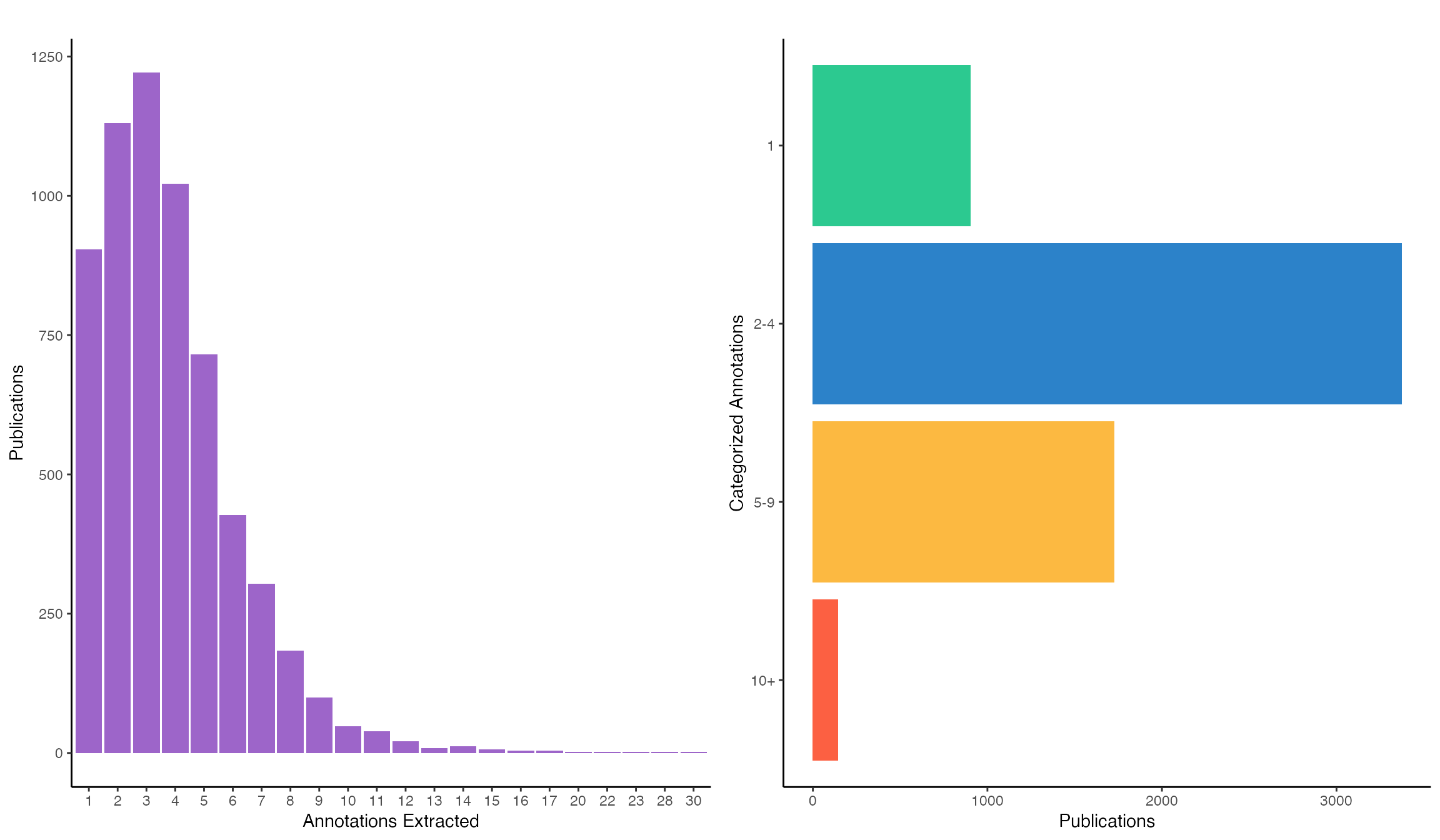
Each publication has a varying number of extracted annotations; therefore, we have binned them into four categories: publications with 1, 2-4, 5-9, or 10+ cell line annotations. Publications with a single annotation are likely to be very specific. While 2-4 and 5-9 are likely studies with multiple validation experiments performed in additional cell lines.

p1 <- table(publications$n_annotations) %>%
      data.frame() %>%
      magrittr::set_colnames(c("annotations", "freq")) %>%
      ggplot(aes(x=annotations, y=freq)) +
        geom_bar(stat="identity", fill="#9d65c9") +
        labs(title="", x="Annotations Extracted", y="Publications") +
        theme_classic() + 
        theme(legend.position="none")

p2 <- table(publications$specificity) %>%
      data.frame() %>%
      magrittr::set_colnames(c("category", "freq")) %>%
      dplyr::mutate(category = factor(category, levels=rev(c("1", "2-4", "5-9", "10+")))) %>%
      ggplot(aes(x=category, y=freq, fill=category)) +
        geom_bar(stat="identity") +
        coord_flip() +
        scale_fill_manual(values = c("1"="#2CC990", "2-4"="#2C82C9", "5-9"="#FCB941", "10+"="#FC6042")) +
        labs(title="", x="Categorized Annotations", y="Publications") +
        theme_classic() + 
        theme(legend.position="none")

ggarrange(p1, p2, ncol=2)

Filtering interactions

ppi <- data.ppi("data/v_1_00/PPI-Context.txt")

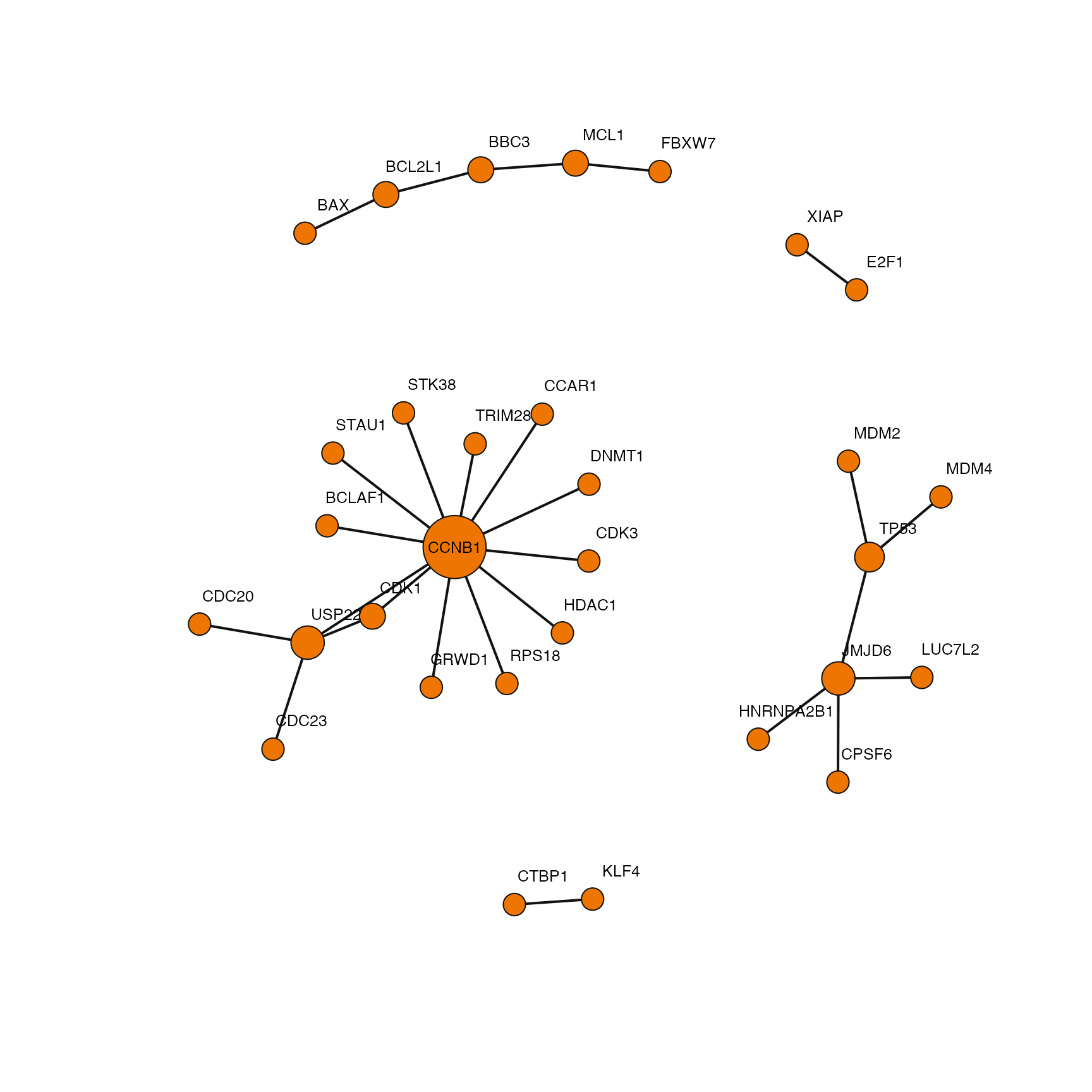
Here is a small example for filtering interactions based on the specificity of their reporting publication. First we isolate PPIs annotated with a given cell line and then filter again by publications with only a single annotation. Lastly we put the interactions into an undirected graph object so we can analyze them as a single network.

ig <- ppi %>%
      dplyr::filter(cell_name == "HCT 116") %>%
      dplyr::filter(pid %in% dplyr::filter(publications, specificity == "1")$pid) %>%
      dplyr::select(gene_a, gene_b) %>%
      magrittr::set_colnames(c("to", "from")) %>%
      igraph::graph_from_data_frame(directed=FALSE) %>%
      igraph::simplify()

plot(ig, 
     vertex.size=degree(ig)+5, 
     vertex.frame.color="gray7",
     vertex.color="darkorange2",
     vertex.label.family="Helvetica", 
     vertex.label.dist=ifelse(degree(ig) > 10, 0, 1.5),
     vertex.label.cex=0.8,
     vertex.label.color="black",
     edge.width=2,
     edge.color="gray7")