Requirements

We recommend the latest version of R (>= 4.0.0) but hypeR currently requires R (>= 3.6.0) to be installed directly from Github or Bioconductor.

Installation

Install the development version of the package from Github.

devtools::install_github("montilab/hypeR")

Or install the development version of the package from Bioconductor.

BiocManager::install("montilab/hypeR", version="devel")

Usage

library(hypeR)
library(tidyverse)
library(reactable)

Data

load(file.path(system.file("extdat", package="hyperworkshop"), "limma.rda"))
load(file.path(system.file("extdat", package="hyperworkshop"), "wgcna.rda"))

signatures <- wgcna[[1]]
str(signatures)

List of 21
 $ turquoise   : chr [1:1902] "CLEC3A" "KCNJ3" "SCGB2A2" "SERPINA6" ...
 $ blue        : chr [1:1525] "GSTM1" "BMPR1B" "BMPR1B-DT" "PYDC1" ...
 $ magenta     : chr [1:319] "DSCAM-AS1" "VSTM2A" "UGT2B11" "CYP4Z1" ...
 $ brown       : chr [1:1944] "SLC25A24P1" "CPB1" "GRIA2" "CST9" ...
 $ pink        : chr [1:578] "MUC6" "GLRA3" "OPRPN" "ARHGAP36" ...
 $ red         : chr [1:681] "KCNC2" "SLC5A8" "HNRNPA1P57" "CBLN2" ...
 $ darkred     : chr [1:43] "OR4K12P" "GRAMD4P7" "FAR2P3" "CXADRP3" ...
 $ tan         : chr [1:161] "LEP" "SIK1" "TRARG1" "CIDEC" ...
 $ lightcyan   : chr [1:82] "CDC20B" "FOXJ1" "CDHR4" "MCIDAS" ...
 $ purple      : chr [1:308] "C10orf82" "GUSBP3" "IGLV10-54" "IGKV1D-13" ...
 $ lightyellow : chr [1:48] "SLC6A4" "ERICH3" "GP2" "TRIM72" ...
 $ cyan        : chr [1:143] "NOP56P1" "FABP6" "GNAQP1" "ZNF725P" ...
 $ royalblue   : chr [1:47] "PCDHA12" "PCDHA11" "PCDHA4" "PCDHA1" ...
 $ black       : chr [1:864] "NSFP1" "USP32P2" "OCLNP1" "RN7SL314P" ...
 $ yellow      : chr [1:904] "NPIPB15" "MAFA-AS1" "C1orf167" "NT5CP2" ...
 $ lightgreen  : chr [1:60] "HIST1H2APS3" "HIST1H2AI" "HIST1H1PS1" "HIST1H3H" ...
 $ darkgrey    : chr [1:34] "MTND4P12" "MTRNR2L1" "MT-TT" "MTCYBP18" ...
 $ darkgreen   : chr [1:43] "STK19B" "SNCG" "ELANE" "TNXA" ...
 $ midnightblue: chr [1:92] "LRRC26" "ARHGDIG" "TGFBR3L" "HS6ST1P1" ...
 $ grey60      : chr [1:71] "KRT8P48" "KRT8P42" "KRT8P11" "CRIP1P4" ...
 $ salmon      : chr [1:151] "UBA52P3" "NPM1P33" "MYL6P5" "RPL29P30" ...

genesets <- msigdb_gsets("Homo sapiens", "C2", "CP:KEGG", clean=TRUE)
print(genesets)

C2.CP:KEGG v7.1.1 
Abc Transporters (44)
Acute Myeloid Leukemia (57)
Adherens Junction (73)
Adipocytokine Signaling Pathway (67)
Alanine Aspartate And Glutamate Metabolism (32)
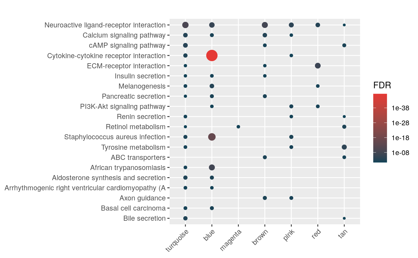
Aldosterone Regulated Sodium Reabsorption (42)

mhyp <- hypeR(signatures, genesets, test="hypergeometric", background=36000)

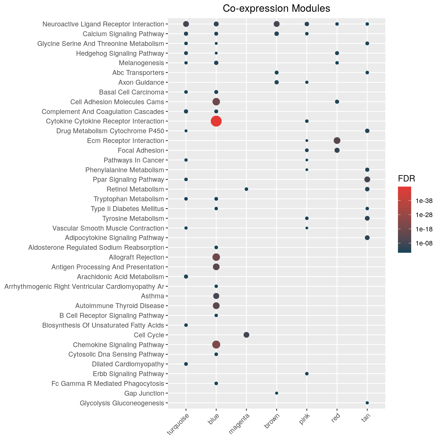
hyp_dots(mhyp, merge=TRUE, fdr=0.05, top=40, title="Co-expression Modules")

Why hypeR?

Written purely in R
Designed to make your life easier
Flexible functionality and parameters
Able to process hundreds of signatures simultaneously
Dynamic visualizations for large amounts of data
Highly reproducible workflows
Report generation for sharing with collaborators

Geneset Enrichment 101

Terminology

All analyses with hypeR must include one or more signatures and genesets.

Signature

There are multiple types of enrichment analyses (e.g. hypergeometric, kstest, gsea) one can perform. Depending on the type, different kinds of signatures are expected. There are three types of signatures hypeR() expects.

# Simply a character vector of symbols (hypergeometric)
signature <- c("GENE1", "GENE2", "GENE3")

# A ranked character vector of symbols (kstest)
ranked.signature <- c("GENE2", "GENE1", "GENE3")

# A ranked named numerical vector of symbols with ranking weights (gsea)
weighted.signature <- c("GENE2"=1.22, "GENE1"=0.94, "GENE3"=0.77)

Geneset

A geneset is simply a list of vectors, therefore, one can use any custom geneset in their analyses, as long as it’s appropriately defined. Additionally, hypeR() recognized object oriented genesets called gsets objects, described later.

genesets <- list("GSET1" = c("GENE1", "GENE2", "GENE3"),
                 "GSET2" = c("GENE4", "GENE5", "GENE6"),
                 "GSET3" = c("GENE7", "GENE8", "GENE9"))

Using a differential expression dataframe created with Limma, we will extract a signature of upregulated genes for use with a hypergeometric test and rank genes descending by their differential expression level for use with a kstest.

reactable(limma, rownames=FALSE)

We’ll also import the latest genesets from Kegg using another set of functions provided by hypeR for downloading and loading hundreds of open source genesets.

genesets <- msigdb_gsets("Homo sapiens", "C2", "CP:KEGG", clean=TRUE)

Enrichment Methods

All workflows begin with performing enrichment with hypeR(). Often we’re just interested in a single signature, as described above. In this case, hypeR() will return a hyp object. This object contains relevant information to the enrichment results, as well as plots for each geneset tested, and is recognized by downstream methods.

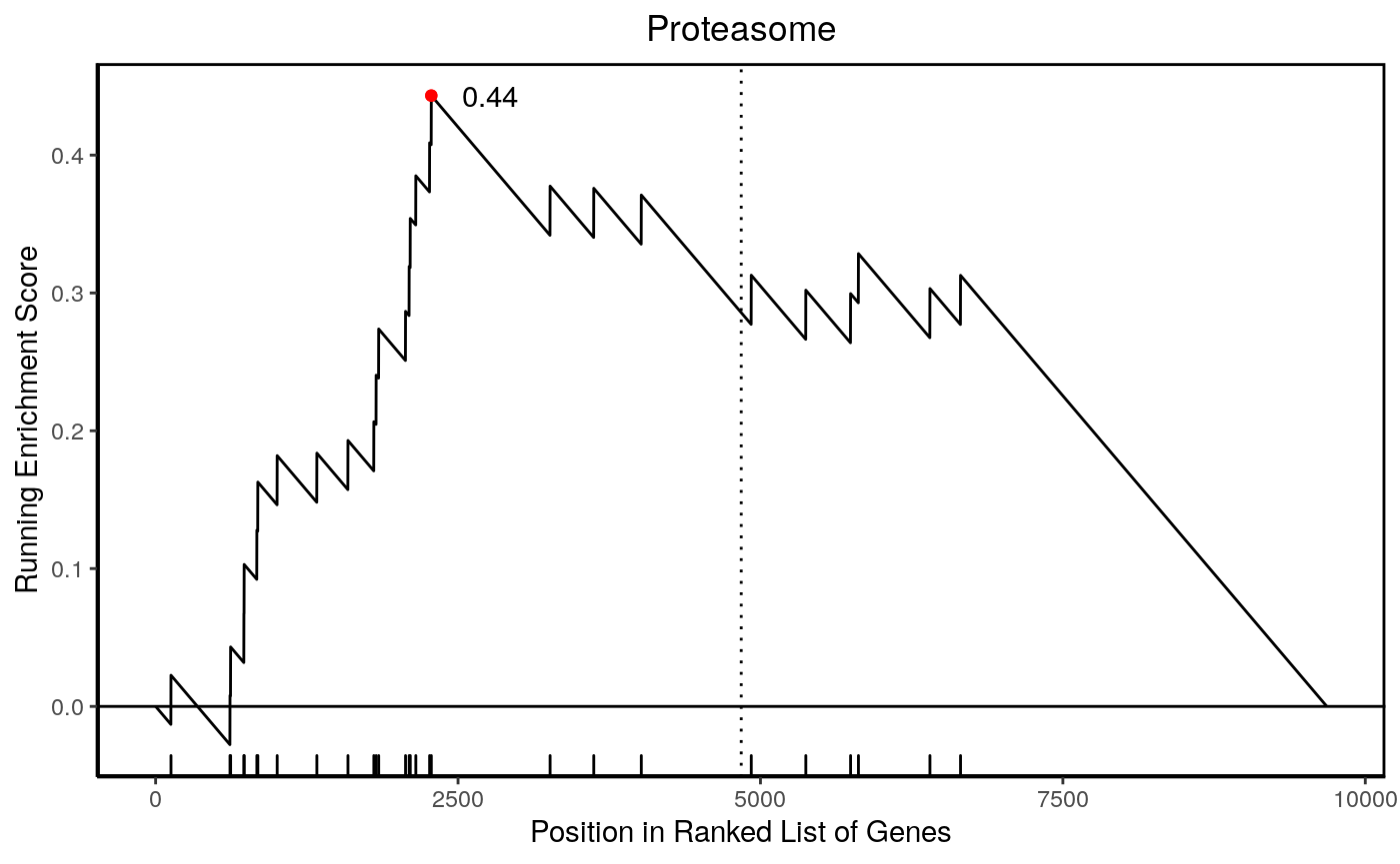
The most basic signature is an unranked vector of genes. This could be a differential expression signature, module of co-expressed genes, etc. As an example, we use the differential expression dataframe to filter genes that are upregulated (t > 0) and are sufficiently significant (fdr < 0.001), then extract the gene symbol column as a vector.

Unranked Signature

signature <- limma %>%
             dplyr::filter(t > 0 & fdr < 0.001) %>%
             magrittr::use_series(symbol)

length(signature)

[1] 213

head(signature)

[1] "LMAN2L" "SHKBP1" "SPHK2"  "AJUBA"  "TJP1"   "TMCC3"

hyp_obj <- hypeR(signature, genesets, test="hypergeometric", background=50000, fdr=0.01, plotting=TRUE)
hyp_obj$plots[[1]]

Ranked Signature

Rather than setting a specific cutoff to define a differential expression signature, one could rank genes by their expression and provide the entire ranked vector as signature. From the differential expression dataframe, we order genes descending so upregulated genes are near the top, then extract the gene symbol column as a vector.

signature <- limma %>%
             dplyr::arrange(desc(t)) %>%
             magrittr::use_series(symbol)

length(signature)

[1] 9682

head(signature)

[1] "LMAN2L" "SHKBP1" "SPHK2"  "AJUBA"  "TJP1"   "TMCC3"

hyp_obj <- hypeR(signature, genesets, test="kstest", fdr=0.05, plotting=TRUE)
hyp_obj$plots[[1]]

Weighted Signature

In addition to providing a ranked signature, one could also add weights by including the t-statistic of the differential expression. From the differential expression dataframe, we order genes descending so upregulated genes are near the top, then extract and deframe the gene symbol and t-statistic columns as a named vector of weights.

signature <- limma %>%
             dplyr::arrange(desc(t)) %>%
             dplyr::select(symbol, t) %>%
             tibble::deframe()

length(signature)

[1] 9682

head(signature)

LMAN2L SHKBP1  SPHK2  AJUBA   TJP1  TMCC3 
  6.59   6.56   6.37   6.26   6.26   6.11

hyp_obj <- hypeR(signature, genesets, test="kstest", fdr=0.05, plotting=TRUE)
hyp_obj$plots[[1]]

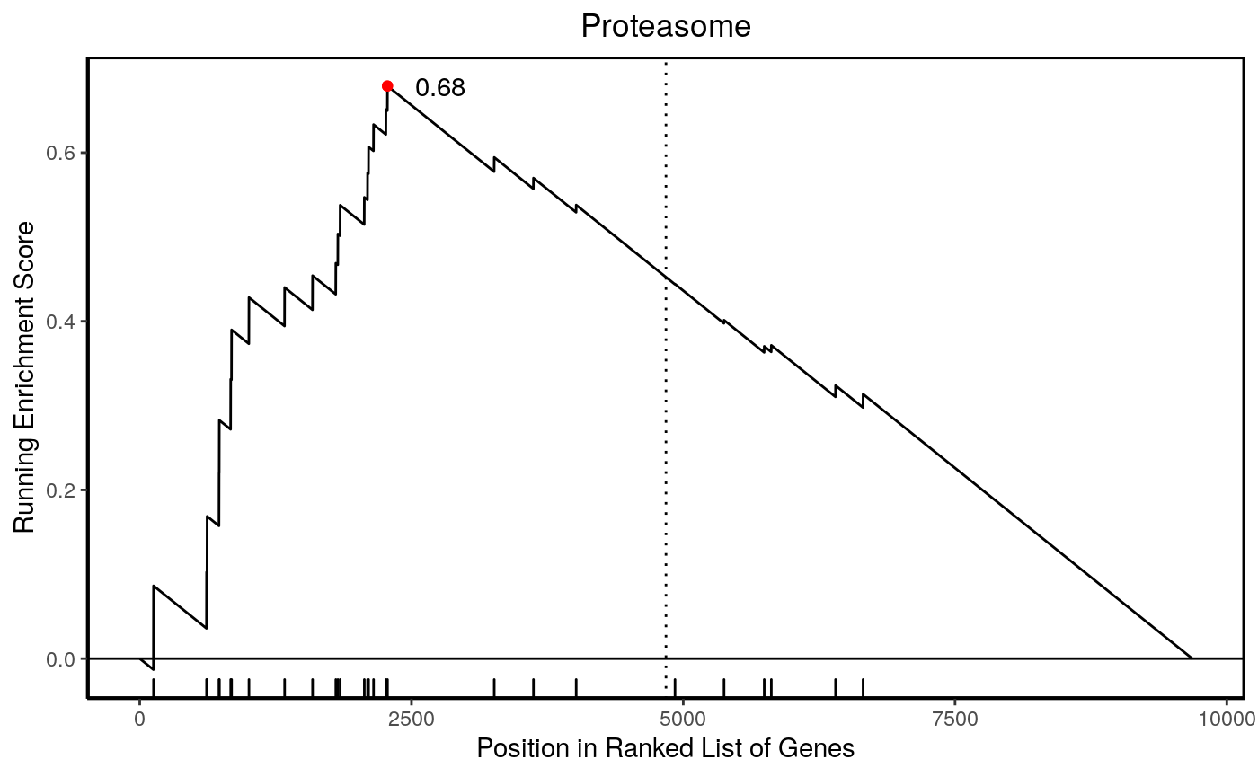
A hyp object contains all information relevant to the enrichment analysis, including the parameters used, a dataframe of results, plots for each geneset tested, as well as the arguments used to perform the analysis. All downstream functions used for analysis, visualization, and reporting recognize hyp objects and utilize their data. Adopting an object oriented framework brings modularity to hypeR, enabling flexible and reproducible workflows.

print(hyp_obj)

(hyp) 

  data: 
                            label    pval    fdr signature geneset overlap
                       Proteasome 1.7e-05 0.0032      9682      46      28
             Steroid Biosynthesis 6.4e-05 0.0060      9682      17      12
                Pancreatic Cancer 1.8e-04 0.0098      9682      70      49
   Neurotrophin Signaling Pathway 2.1e-04 0.0098      9682     126      87
 Fc Gamma R Mediated Phagocytosis 4.8e-04 0.0180      9682      96      62
             Renal Cell Carcinoma 6.6e-04 0.0200      9682      70      47
 score
  0.44
  0.63
  0.30
  0.22
  0.25
  0.28

  plots: 11 Figures

  args: signature
        genesets
        test
        background
        power
        absolute
        pval
        fdr
        plotting
        quiet

The `hyp` Methods

# Show interactive table
hyp_show(hyp_obj)

# Plot dots plot
hyp_dots(hyp_obj)

# Plot enrichment map
hyp_emap(hyp_obj)

# Plot hiearchy map
hyp_hmap(hyp_obj)

# Save to excel
hyp_to_excel(hyp_obj)

# Save to table
hyp_to_table(hyp_obj)

# Generate markdown report
hyp_to_rmd(hyp_obj)

Downloading Genesets

Object Oriented Genesets

Genesets are simply a named list of character vectors which can be directly passed to hyper(). Alternatively, one can pass a gsets object, which can retain the name and version of the genesets one uses. This versioning will be included when exporting results or generating reports, which will ensure your results are reproducible.

genesets <- list("GSET1" = c("GENE1", "GENE2", "GENE3"),
                 "GSET2" = c("GENE4", "GENE6"),
                 "GSET3" = c("GENE7", "GENE8", "GENE9"))

Creating a gsets object is easy…

genesets <- gsets$new(genesets, name="Example Genesets", version="v1.0")
print(genesets)

Example Genesets v1.0 
GSET1 (3)
GSET2 (2)
GSET3 (3)

And can be passed directly to hyper()…

hypeR(signature, genesets)

To aid in workflow efficiency, hypeR enables users to download genesets, wrapped as gsets objects, from multiple data sources.

Downloading msigdb Genesets

Most researchers will find the genesets hosted by msigdb are adequate to perform geneset enrichment analysis. There are various types of genesets available across multiple species.

msigdb_info()

|------------------------------------------------------------------|
| Via: R package msigdbr                                    v7.1.1 |
|------------------------------------------------------------------|
| Available Species                                                |
|------------------------------------------------------------------|
| Homo sapiens                                                     |
| Mus musculus                                                     |
| Drosophila melanogaster                                          |
| Gallus gallus                                                    |
| Saccharomyces cerevisiae                                         |
| Bos taurus                                                       |
| Caenorhabditis elegans                                           |
| Canis lupus familiaris                                           |
| Danio rerio                                                      |
| Rattus norvegicus                                                |
| Sus scrofa                                                       |
|------------------------------------------------------------------|
| Available Genesets                                               |
|------------------------------------------------------------------|
| Category Subcategory | Description                               |
|------------------------------------------------------------------|
| C1                   | Positional                                |
| C2 CGP               | Chemical and Genetic Perturbations        |
| C2 CP                | Canonical Pathways                        |
| C2 CP:BIOCARTA       | Canonical BIOCARTA                        |
| C2 CP:KEGG           | Canonical KEGG                            |
| C2 CP:PID            | Canonical PID                             |
| C2 CP:REACTOME       | Canonical REACTOME                        |
| C3 MIR               | Motif miRNA Targets                       |
| C3 TFT               | Motif Transcription Factor Targets        |
| C4 CGN               | Cancer Gene Neighborhoods                 |
| C4 CM                | Cancer Modules                            |
| C5 BP                | GO Biological Process                     |
| C5 CC                | GO Cellular Component                     |
| C5 MF                | GO Molecular Function                     |
| C6                   | Oncogenic Signatures                      |
| C7                   | Immunologic Signatures                    |
| H                    | Hallmark                                  |
|------------------------------------------------------------------|
| Source: http://software.broadinstitute.org/gsea/msigdb           |
|------------------------------------------------------------------|

Here we download the Hallmarks genesets…

HALLMARK <- msigdb_gsets(species="Homo sapiens", category="H")
print(HALLMARK)

H v7.1.1 
HALLMARK_ADIPOGENESIS (200)
HALLMARK_ALLOGRAFT_REJECTION (200)
HALLMARK_ANDROGEN_RESPONSE (100)
HALLMARK_ANGIOGENESIS (36)
HALLMARK_APICAL_JUNCTION (200)
HALLMARK_APICAL_SURFACE (44)

We can also clean them up by removing the first leading common substring…

HALLMARK <- msigdb_gsets(species="Homo sapiens", category="H", clean=TRUE)
print(HALLMARK)

H v7.1.1 
Adipogenesis (200)
Allograft Rejection (200)
Androgen Response (100)
Angiogenesis (36)
Apical Junction (200)
Apical Surface (44)

This can be passed directly to hypeR()…

hypeR(signature, genesets=HALLMARK)

Other commonly used genesets include Biocarta, Kegg, and Reactome…

BIOCARTA <- msigdb_gsets(species="Homo sapiens", category="C2", subcategory="CP:BIOCARTA")
KEGG     <- msigdb_gsets(species="Homo sapiens", category="C2", subcategory="CP:KEGG")
REACTOME <- msigdb_gsets(species="Homo sapiens", category="C2", subcategory="CP:REACTOME")

Downloading enrichr Genesets

If msigdb genesets are not sufficient, we have also provided another set of functions for downloading and loading other publicly available genesets. This is facilitated by interfacing with the publicly available libraries hosted by enrichr.

available <- enrichr_available()
reactable(available)

KEGG <- enrichr_gsets("KEGG_2019_Human")
print(KEGG)

KEGG_2019_Human (Enrichr) Downloaded: 2020-07-28 
ABC transporters (45)
AGE-RAGE signaling pathway in diabetic complications (100)
AMPK signaling pathway (120)
Acute myeloid leukemia (66)
Adherens junction (72)
Adipocytokine signaling pathway (69)

Note: These libraries do not have a systematic versioning scheme, however the date downloaded will be recorded.

Additionally download other species if you aren’t working with human or mouse genes!

yeast <- enrichr_gsets("GO_Biological_Process_2018", db="YeastEnrichr")
worm <- enrichr_gsets("GO_Biological_Process_2018", db="WormEnrichr")
fish <- enrichr_gsets("GO_Biological_Process_2018", db="FishEnrichr")
fly <- enrichr_gsets("GO_Biological_Process_2018", db="FlyEnrichr")

Visualization

signature <- limma %>%
             dplyr::arrange(desc(t)) %>%
             magrittr::use_series(symbol)

head(signature)

[1] "LMAN2L" "SHKBP1" "SPHK2"  "AJUBA"  "TJP1"   "TMCC3"

genesets <- msigdb_gsets("Homo sapiens", "C2", "CP:REACTOME", clean=TRUE)

hyp_obj <- hypeR(signature, genesets, test="kstest", fdr=0.01)

To visualize the results, just pass the hyp object to any downstream functions.

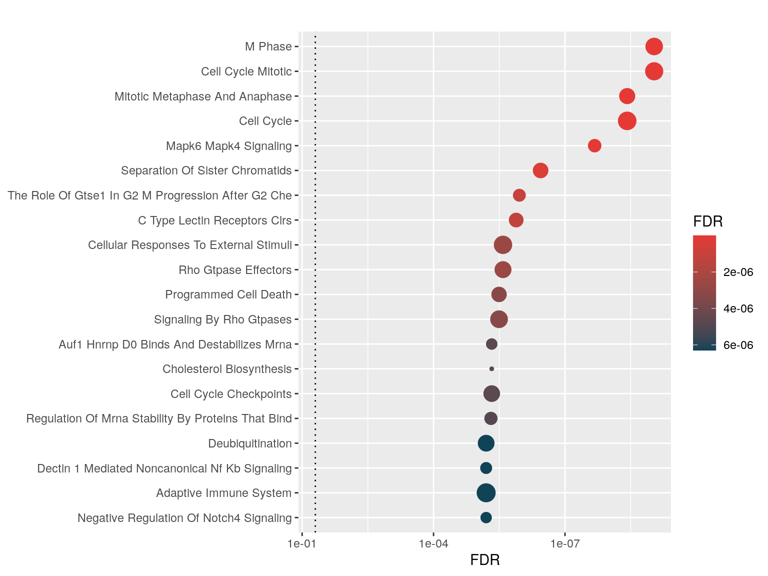
Dots Plot

One can visualize the top enriched genesets using hyp_dots() which returns a horizontal dots plot. Each dot is a geneset, where the color represents the significance and the size signifies the geneset size.

hyp_dots(hyp_obj)

Enrichment Map

One can visualize the top enriched genesets using hyp_emap() which will return an enrichment map. Each node represents a geneset, where the shade of red indicates the normalized significance of enrichment. Hover over the node to view the raw value. Edges represent geneset similarity, calculated by either jaccard or overlap similarity metrics.

hyp_emap(hyp_obj, similarity_cutoff=0.70)

Hiearchy Map

When dealing with hundreds of genesets, it’s often useful to understand the relationships between them. This allows researchers to summarize many enriched pathways as more general biological processes. To do this, we rely on curated relationships defined between them.

Relational Genesets

For example, Reactome conveniently defines their genesets in a hiearchy of pathways. This data can be formatted into a relational genesets object called rgsets.

genesets <- hyperdb_rgsets("REACTOME", version="70.0")

Relational genesets have three data atrributes including gsets, nodes, and edges. The genesets attribute includes the geneset information for the leaf nodes of the hiearchy, the nodes attribute describes all nodes in the hierarchy, including internal nodes, and the edges attribute describes the edges in the hiearchy.

print(genesets)

REACTOME v70.0 

Genesets

2-LTR circle formation (13)
5-Phosphoribose 1-diphosphate biosynthesis (3)
A tetrasaccharide linker sequence is required for GAG synthesis (26)
ABC transporters in lipid homeostasis (18)
ABO blood group biosynthesis (3)
ADP signalling through P2Y purinoceptor 1 (25)

Nodes

                                                                        label
R-HSA-164843                                           2-LTR circle formation
R-HSA-73843                        5-Phosphoribose 1-diphosphate biosynthesis
R-HSA-1971475 A tetrasaccharide linker sequence is required for GAG synthesis
R-HSA-5619084                                       ABC transporter disorders
R-HSA-1369062                           ABC transporters in lipid homeostasis
R-HSA-382556                           ABC-family proteins mediated transport
                         id length
R-HSA-164843   R-HSA-164843     13
R-HSA-73843     R-HSA-73843      3
R-HSA-1971475 R-HSA-1971475     26
R-HSA-5619084 R-HSA-5619084     77
R-HSA-1369062 R-HSA-1369062     18
R-HSA-382556   R-HSA-382556     22

Edges

          from            to
1 R-HSA-109581  R-HSA-109606
2 R-HSA-109581  R-HSA-169911
3 R-HSA-109581 R-HSA-5357769
4 R-HSA-109581   R-HSA-75153
5 R-HSA-109582  R-HSA-140877
6 R-HSA-109582  R-HSA-202733

Passing relational genesets works natively with hypeR().

hyp_obj <- hypeR(signature, genesets, test="kstest", fdr=0.01)

One can visualize the top enriched genesets using hyp_hmap() which will return a hiearchy map. Each node represents a geneset, where the shade of the gold border indicates the normalized significance of enrichment. Hover over the leaf nodes to view the raw value. Double click internal nodes to cluster their first degree connections. Edges represent a directed relationship between genesets in the hiearchy. Note: This function only works when the hyp object was inialized with an rgsets object.

hyp_hmap(hyp_obj, top=30)

Use Case: Gene Co-Expression Analysis

Often computational biologists must process, interpret, and share large amounts of biological data. A common example is interpreting gene co-expression modules across one or more phenotype, resulting in potentially hundreds of signatures to annotate. Here we have signatures of gene co-expression modules, generated with WGCNA, for multiple breast cancer subtypes

Problem: Annotate gene co-expression modules across one or more phenotype, resulting in potentially hundreds of signatures to annotate. ## Example Data

We’re using publicly available RNA-seq data from breast cancer samples from The Cancer Genome Atlas. The data has been normalized with DESeq2, log-transformed, and subtyped using PAM50 signatures.

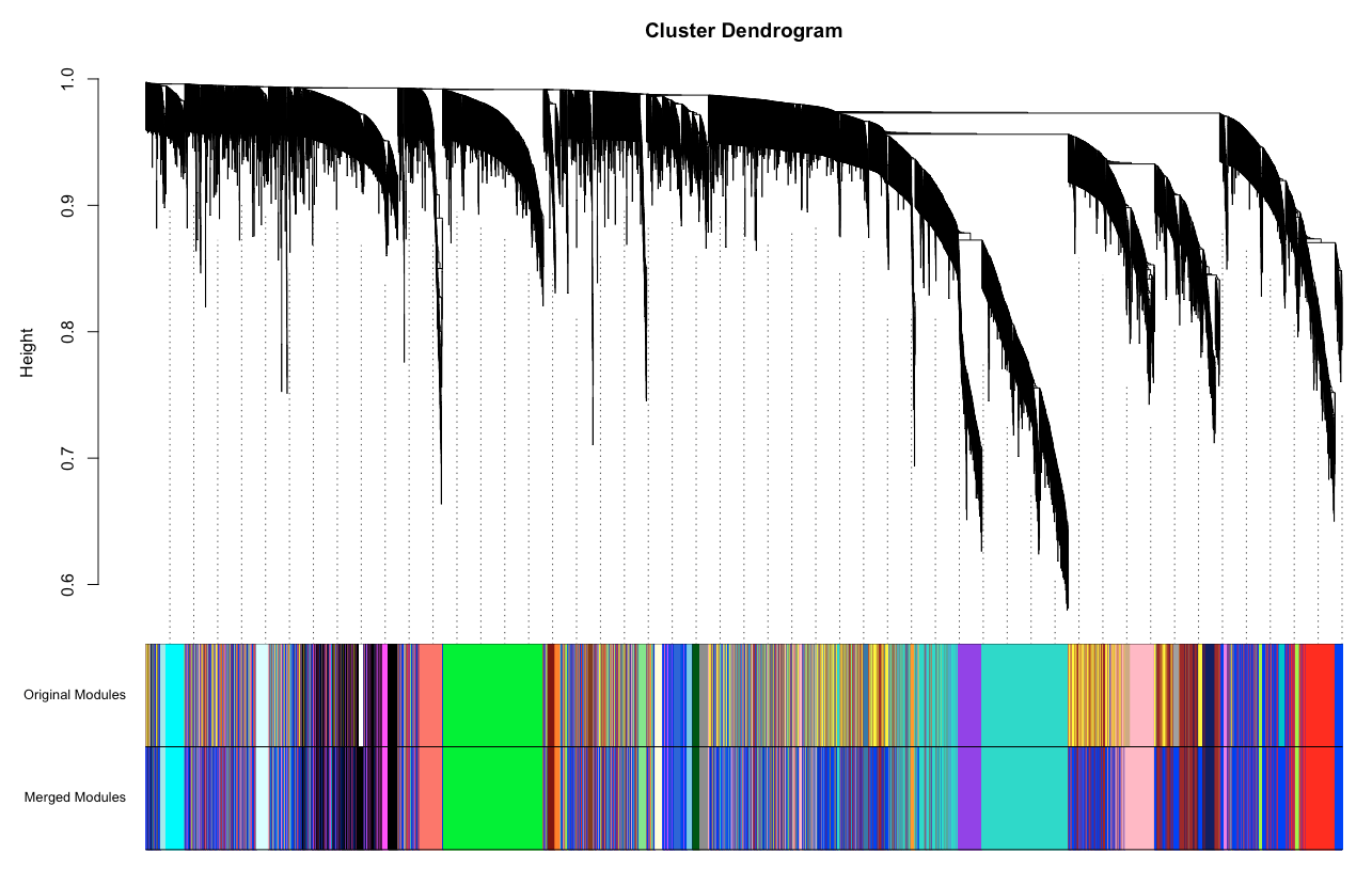
brca <- readRDS("data/TCGA-BRCA-RNA-Seq-Expression-Set.rds")
dim(brca)

Weighted Gene Co-Expression Analysis (WGCNA)

run.wgcna(brca)

Apply to BRCA Subtypes

Isolate tumor samples with subtypes LumA, LumB, Her2, and Basal.

subtypes <- c("LA", "LB", "H2", "BL")
brca.tumors <- brca[, brca$subtype %in% subtypes]
table(brca.tumors$subtype)

wgcna <- list("LA" = run.wgcna(brca.tumors, subtype="LA"),
              "LB" = run.wgcna(brca.tumors, subtype="LB"),
              "H2" = run.wgcna(brca.tumors, subtype="H2"),
              "BL" = run.wgcna(brca.tumors, subtype="BL"))

Resulting 87 Signatures to Annotate…

str(wgcna)

List of 4
 $ LA:List of 21
  ..$ turquoise   : chr [1:1902] "CLEC3A" "KCNJ3" "SCGB2A2" "SERPINA6" ...
  ..$ blue        : chr [1:1525] "GSTM1" "BMPR1B" "BMPR1B-DT" "PYDC1" ...
  ..$ magenta     : chr [1:319] "DSCAM-AS1" "VSTM2A" "UGT2B11" "CYP4Z1" ...
  ..$ brown       : chr [1:1944] "SLC25A24P1" "CPB1" "GRIA2" "CST9" ...
  ..$ pink        : chr [1:578] "MUC6" "GLRA3" "OPRPN" "ARHGAP36" ...
  ..$ red         : chr [1:681] "KCNC2" "SLC5A8" "HNRNPA1P57" "CBLN2" ...
  ..$ darkred     : chr [1:43] "OR4K12P" "GRAMD4P7" "FAR2P3" "CXADRP3" ...
  ..$ tan         : chr [1:161] "LEP" "SIK1" "TRARG1" "CIDEC" ...
  ..$ lightcyan   : chr [1:82] "CDC20B" "FOXJ1" "CDHR4" "MCIDAS" ...
  ..$ purple      : chr [1:308] "C10orf82" "GUSBP3" "IGLV10-54" "IGKV1D-13" ...
  ..$ lightyellow : chr [1:48] "SLC6A4" "ERICH3" "GP2" "TRIM72" ...
  ..$ cyan        : chr [1:143] "NOP56P1" "FABP6" "GNAQP1" "ZNF725P" ...
  ..$ royalblue   : chr [1:47] "PCDHA12" "PCDHA11" "PCDHA4" "PCDHA1" ...
  ..$ black       : chr [1:864] "NSFP1" "USP32P2" "OCLNP1" "RN7SL314P" ...
  ..$ yellow      : chr [1:904] "NPIPB15" "MAFA-AS1" "C1orf167" "NT5CP2" ...
  ..$ lightgreen  : chr [1:60] "HIST1H2APS3" "HIST1H2AI" "HIST1H1PS1" "HIST1H3H" ...
  ..$ darkgrey    : chr [1:34] "MTND4P12" "MTRNR2L1" "MT-TT" "MTCYBP18" ...
  ..$ darkgreen   : chr [1:43] "STK19B" "SNCG" "ELANE" "TNXA" ...
  ..$ midnightblue: chr [1:92] "LRRC26" "ARHGDIG" "TGFBR3L" "HS6ST1P1" ...
  ..$ grey60      : chr [1:71] "KRT8P48" "KRT8P42" "KRT8P11" "CRIP1P4" ...
  ..$ salmon      : chr [1:151] "UBA52P3" "NPM1P33" "MYL6P5" "RPL29P30" ...
 $ LB:List of 22
  ..$ turquoise   : chr [1:5327] "CLEC3A" "PSPHP1" "PRAME" "CPB1" ...
  ..$ black       : chr [1:195] "TFAP2B" "MUC5B" "ZIC2" "CRABP1" ...
  ..$ blue        : chr [1:2282] "SCGB2A2" "KCNJ3" "ASCL1" "CGA" ...
  ..$ magenta     : chr [1:161] "BEX1" "ONECUT2" "SULT4A1" "PCSK1N" ...
  ..$ red         : chr [1:199] "PVALB" "PIP" "SERPINA6" "COL2A1" ...
  ..$ purple      : chr [1:151] "ADIPOQ" "TRARG1" "ADH1B" "CIDEC" ...
  ..$ cyan        : chr [1:70] "KRT14" "KRT6B" "KRT5" "KLK5" ...
  ..$ salmon      : chr [1:85] "PCDHA11" "PCDHA12" "DIO1" "PCDHA4" ...
  ..$ lightcyan   : chr [1:59] "CDC20B" "FOXJ1" "MCIDAS" "CCNO" ...
  ..$ yellow      : chr [1:244] "TPSG1" "PRTN3" "PYY" "AZU1" ...
  ..$ royalblue   : chr [1:46] "DLGAP1" "OR7E22P" "PTPRN2" "DCX" ...
  ..$ lightgreen  : chr [1:56] "HIST1H3G" "HIST1H2APS3" "HIST1H1D" "HIST1H2AI" ...
  ..$ midnightblue: chr [1:68] "B3GALT5" "PCP4" "B3GALT5-AS1" "IFI27" ...
  ..$ pink        : chr [1:166] "PNMT" "TBX1" "MAPK15" "KRT13" ...
  ..$ lightyellow : chr [1:49] "LINC02593" "SAMD11" "EFNA2" "ARHGDIG" ...
  ..$ darkgreen   : chr [1:31] "DOK7" "ITPKA" "CACNA1F" "NHLRC4" ...
  ..$ green       : chr [1:230] "GAPDHP1" "RPS14P8" "MT-TV" "GAPDHP35" ...
  ..$ greenyellow : chr [1:122] "FAM169A" "MIR4768" "ERVE-1" "RPS23P6" ...
  ..$ brown       : chr [1:273] "PWAR5" "SPATA46" "MTND1P8" "EML5" ...
  ..$ tan         : chr [1:88] "GCGR" "TRIM54" "CYP2E1" "GOLGA8A" ...
  ..$ grey60      : chr [1:57] "KRT8P42" "KRT8P48" "KRT8P11" "KRT8P3" ...
  ..$ darkred     : chr [1:41] "ATP1A2" "PCDH19" "ADRA1A" "FRAS1" ...
 $ H2:List of 25
  ..$ blue         : chr [1:1940] "CLEC3A" "S100A7" "CYP2B7P" "CASP14" ...
  ..$ orange       : chr [1:631] "GSTM1" "RPSAP53" "LINC01833" "LINC00461" ...
  ..$ brown        : chr [1:885] "SLC5A8" "DSCAM-AS1" "PRAME" "KCNJ3" ...
  ..$ darkred      : chr [1:54] "NXPH1" "PNMT" "SCGN" "GACAT3" ...
  ..$ green        : chr [1:586] "ARHGAP40" "CYP4F8" "GATD3A" "IRX4" ...
  ..$ darkgreen    : chr [1:49] "MUCL1" "BRINP3" "C2CD4A" "DMRTC2" ...
  ..$ turquoise    : chr [1:2389] "MKRN3" "MUC6" "SOX2" "GUSBP3" ...
  ..$ cyan         : chr [1:137] "HMGCS2" "ONECUT2" "PLAC9P1" "SLC7A4" ...
  ..$ salmon       : chr [1:178] "PYDC1" "PCDHB2" "LINC01342" "ARHGDIG" ...
  ..$ lightyellow  : chr [1:65] "ABCC12" "LRRC31" "MUC19" "CEACAM5" ...
  ..$ black        : chr [1:554] "TRARG1" "ADIPOQ" "CIDEA" "CIDEC" ...
  ..$ tan          : chr [1:201] "OLFM4" "TCN1" "KLK11" "CALML3" ...
  ..$ red          : chr [1:578] "PCDHA11" "PCDHA12" "PCDHA4" "USP32P1" ...
  ..$ darkgrey     : chr [1:36] "FOXJ1" "CDC20B" "LRRIQ1" "CCNO" ...
  ..$ royalblue    : chr [1:60] "HIST1H3G" "HIST1H2APS3" "HIST1H2APS4" "HIST1H1D" ...
  ..$ lightcyan    : chr [1:118] "PCSK1N" "ZNF725P" "NCAM2" "RP1" ...
  ..$ grey60       : chr [1:90] "LRRC26" "AMH" "TGFBR3L" "LKAAEAR1" ...
  ..$ magenta      : chr [1:357] "ZSCAN1" "HDGFP1" "PRSS29P" "LINC00930" ...
  ..$ darkturquoise: chr [1:49] "DYDC2" "ATP6V1B1" "PRSS50" "PRSS45" ...
  ..$ pink         : chr [1:453] "SPATA46" "ZNF727" "XIST" "ZSCAN23" ...
  ..$ midnightblue : chr [1:127] "ADGRV1" "LINC02211" "LRRC37A9P" "CCDC144B" ...
  ..$ lightgreen   : chr [1:90] "FAM90A2P" "VN1R5" "FAM71F1" "NXF5" ...
  ..$ white        : chr [1:32] "ELANE" "CFD" "C2CD4C" "GSC" ...
  ..$ darkorange   : chr [1:33] "ITPKA" "C20orf204" "STXBP5L" "SULT2B1" ...
  ..$ purple       : chr [1:308] "MTND4P24" "MTRNR2L1" "GAPDHP68" "RPL7P16" ...
 $ BL:List of 19
  ..$ yellow     : chr [1:801] "ADIPOQ" "ADH1B" "GABRA5" "LINP1" ...
  ..$ pink       : chr [1:128] "KRT81" "LINC00518" "VXN" "MUC15" ...
  ..$ purple     : chr [1:75] "S100A7" "CASP14" "KRT6C" "TMPRSS4" ...
  ..$ blue       : chr [1:2280] "CDH19" "LINC01667" "LINC01224" "HILS1" ...
  ..$ turquoise  : chr [1:4149] "FDCSP" "HOXC12" "COL2A1" "AFAP1-AS1" ...
  ..$ grey60     : chr [1:53] "DSG3" "KLK11" "SCEL" "KLK7" ...
  ..$ brown      : chr [1:988] "PEG3" "KLHL34" "SERPINB4" "ZIM2-AS1" ...
  ..$ cyan       : chr [1:63] "KIF1A" "PRDM13" "LINC01606" "TCEAL2" ...
  ..$ lightcyan  : chr [1:57] "CXCL17" "ODAM" "BMP5" "ART3" ...
  ..$ tan        : chr [1:67] "SLC6A15" "ALX1" "KCNV1" "MYO3A" ...
  ..$ green      : chr [1:427] "CALML5" "GSTM1" "PRAC2" "PSPHP1" ...
  ..$ magenta    : chr [1:126] "WIF1" "PRSS33" "COL9A1" "SCRG1" ...
  ..$ red        : chr [1:277] "MINOS1P3" "COX6CP1" "RPL10P6" "ZBTB8OSP2" ...
  ..$ lightyellow: chr [1:46] "IRX4" "RSPO4" "LHX2" "MGAT5B" ...
  ..$ greenyellow: chr [1:69] "IVL" "KRT6A" "LY6D" "KRT4" ...
  ..$ salmon     : chr [1:66] "CEACAM6" "SLURP1" "S100P" "LCN2" ...
  ..$ royalblue  : chr [1:36] "MTND4P24" "MTND1P23" "MTATP8P2" "MT-TT" ...
  ..$ black      : chr [1:246] "GAPDHP1" "GAPDHP35" "RPS14P8" "RPL26P37" ...
  ..$ lightgreen : chr [1:46] "HIST1H2APS3" "HIST1H3C" "HIST1H3A" "HIST1H2AE" ...

Processing Multiple Signatures

We can feed hypeR() one or more signatures. In the case of multiple signatures, a multihyp object will be returned. This object is essentially just multiple hyp objects. However it is recognized and handled differently by downstream methods. Lets start by annotating signatures for the first subtype.

genesets <- msigdb_gsets(species="Homo sapiens", category="C2", subcategory="CP:REACTOME", clean=TRUE)
mhyp <- hypeR(wgcna[["LA"]], genesets=genesets, background=36812, fdr=0.25)

print(mhyp)

(multihyp) 
  (hyp) turquoise
        118 x 8
  (hyp) blue
        121 x 8
  (hyp) magenta
        67 x 8
  (hyp) brown
        59 x 8
  (hyp) pink
        94 x 8
  (hyp) red
        97 x 8
  (hyp) darkred
        0 x 8
  (hyp) tan
        62 x 8
  (hyp) lightcyan
        0 x 8
  (hyp) purple
        28 x 8
  (hyp) lightyellow
        0 x 8
  (hyp) cyan
        0 x 8
  (hyp) royalblue
        0 x 8
  (hyp) black
        0 x 8
  (hyp) yellow
        5 x 8
  (hyp) lightgreen
        0 x 8
  (hyp) darkgrey
        0 x 8
  (hyp) darkgreen
        0 x 8
  (hyp) midnightblue
        0 x 8
  (hyp) grey60
        0 x 8
  (hyp) salmon
        0 x 8

Alternatively, we can pass a background distribution of genes, which will reduce genesets only to the genes used to generate the signatures.

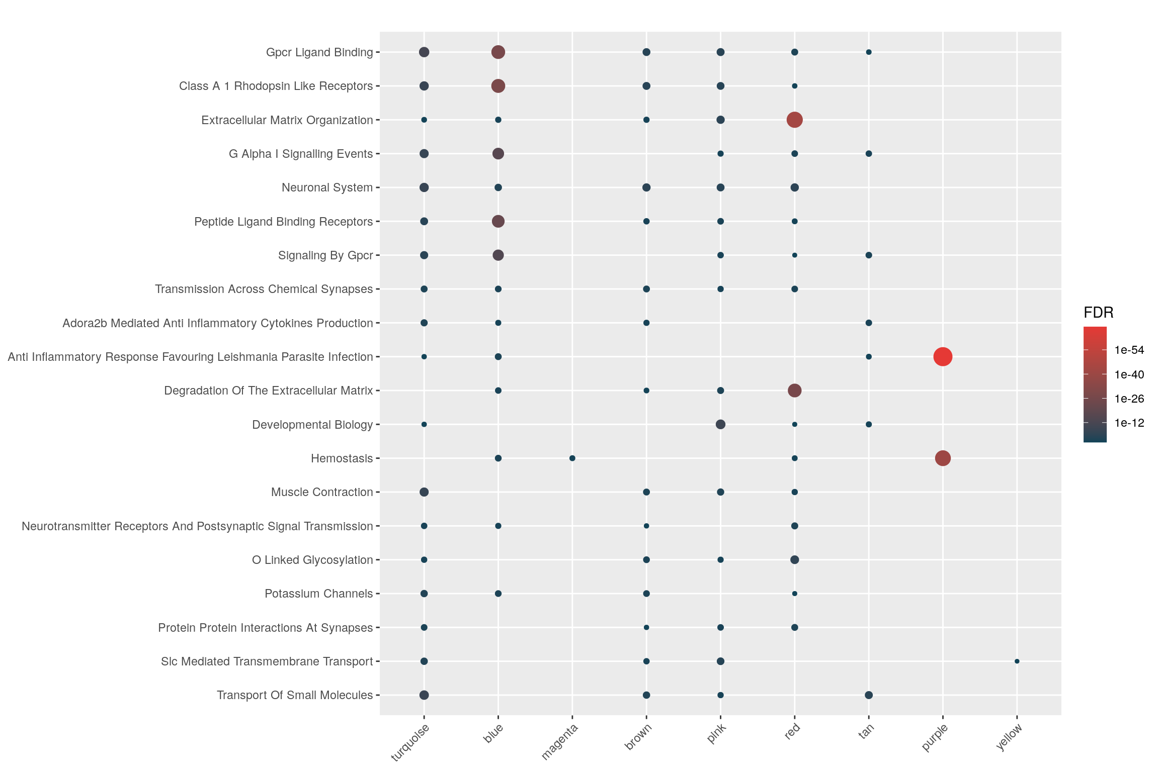
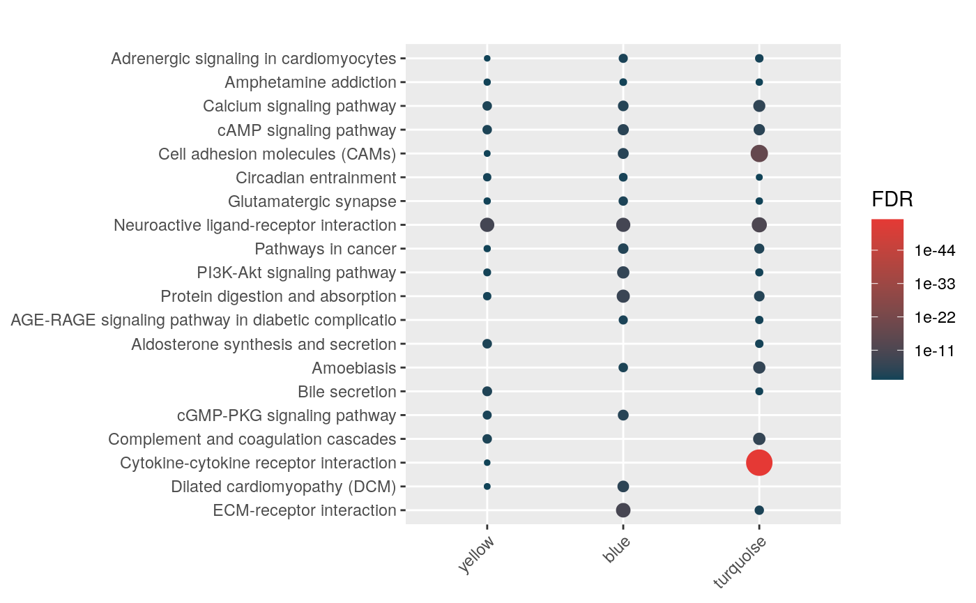
mhyp <- hypeR(wgcna[["LA"]], genesets=genesets, background=rownames(brca), fdr=0.25)

Let’s see the overall enrichment across signatures…

hyp_dots(mhyp, abrv=100, merge=TRUE)

Exporting Results

With hyp_to_table each signature is exported as its own table in a single directory…

hyp_to_table(mhyp, file_path="hypeR")

With hyp_to_excel each signature is exported to its own sheet…

hyp_to_excel(mhyp, file_path="hypeR.xlsx")

A Note on Reproducibility

When data is exported, hypeR makes sure to include all parameters and versioning required for reproducibility.

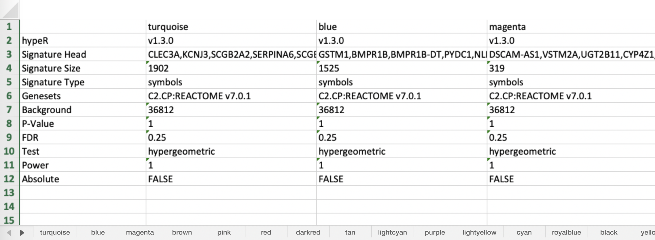
In the case of exporting tables, reproducibility information is in the header of each signature…

#hypeR            v1.3.0
#Signature Head   CLEC3A,KCNJ3,SCGB2A2,SERPINA6,SCGB1D2,RPSAP53
#Signature Size   1902
#Signature Type   symbols
#Genesets         C2.CP:REACTOME v7.0.1
#Background       36812
#P-Value          1
#FDR              0.25
#Test             hypergeometric
#Power            1
#Absolute         FALSE

For excel sheets, there is a dedicated tab with reproducibility information for all signatures…

Generating Reports

Often researchers need to annotate multiple signatures across multiple experiments. Typically, the best way to manage this data is to process it all at once and generate a markdown report to analyze and share with collaborators. Let’s take an example where we have one experiment with many signatures.

In the current example, we want to annotate dozens of co-expression modules for multiple breast cancer subtypes. We have included some convenient functions that return some html for turning hyp and mhyp objects into concise tables for markdown documents. These tables can also include some plots for each individual hyp object.

rctbl_mhyp(mhyp)

Alright, how about we process all of these nested signatures and provide an example of what your markdown report might look like. Because we have a nested list of signatures, we use hyper() with the lapply function. This results in a list of mhyp objects.

genesets <- hyperdb_rgsets("KEGG", "92.0")
lmhyp <- lapply(wgcna, hypeR, genesets, test="hypergeometric", background=36000, fdr=0.05)

First start with a nice theme and include the css required to make the tables pretty.

title: "Project Title"
subtitle: "Project Subtitle"
author: "Anthony Federico"
date: "Last Modified: 'r Sys.Date()'"
output:
  html_document:
    theme: flatly
    toc: true
    toc_float: false
    code_folding: hide
    toc_depth: 4
    css: 'r system.file("style", "rctbl.css", package="hypeR")'

LA

hyp_dots(lmhyp$LA, merge=TRUE)

rctbl_mhyp(lmhyp$LA, show_hmaps=TRUE)

LB

hyp_dots(lmhyp$LB, merge=TRUE)

rctbl_mhyp(lmhyp$LB, show_hmaps=TRUE)

H2

hyp_dots(lmhyp$H2, merge=TRUE)

rctbl_mhyp(lmhyp$H2, show_hmaps=TRUE)

BL

hyp_dots(lmhyp$BL, merge=TRUE)

rctbl_mhyp(lmhyp$BL, show_hmaps=TRUE)

For quick report generation one can use hyp_to_rmd() which will accept multiple formats, including a single hyp or multihyp object as well as a list of either, including a list of hyp or multihyp objects together. When a list of multihyp objects are passed for example, each experiment will become its own section, while each signature becomes its own tab within that section. Lists of keyword arguments can be passed for hyp_dots(), hyp_emap(), and hyp_hmap(), allowing customization of their functionality per report. See hyp_to_rmd() for details.

hyp_to_rmd(lmultihyp_obj,
           file_path="hypeR.rmd",
           title="hypeR Report",
           subtitle="Weighted Gene Co-expression Analysis",
           author="Anthony Federico, Stefano Monti",
           show_dots=T,
           show_emaps=T,
           show_hmaps=T,
           show_tables=T)

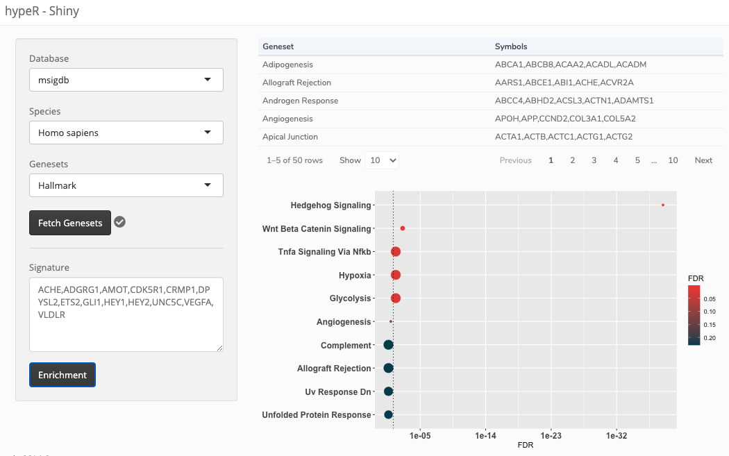
Shiny Modules

All hypeR methods output objects that are compatible with R Shiny and can be incorporated into a variety of applications (e.g. hyp_dots() returns a ggplot object). The most difficult challenge in incorporating geneset enrichment tasks in Shiny applications is the geneselect selection / fetching itself. To help with this, hypeR includes module functions that abstract away the geneset selection code.

What Are Shiny Modules?

Shiny modules are functions that generato Shiny UI / Server code. They are composable elements that can be used within and interface with existing applications. For more information, check out the latest documentation.

Example

For those familiar with Shiny, you will have accompanying modules for the ui and server sections of your application. These modules are hypeR::genesets_UI() and hypeR::genesets_Server() respectively.

UI

Here we create a simple interface where we use the genesets selection module. Through that module, users can select genesets available through hypeR and the application will load those genesets into a reactive variable (more on this later). We add additional code to take a user-defined gene signature and produce an enrichment plot which represents components specific to your Shiny application. This can be anything!

ui <- fluidPage(
        sidebarLayout(
            sidebarPanel(
                # Put your geneset selector module anywhere
                hypeR::genesets_UI("genesets"),

                # Add components specific to your application
                textAreaInput("signature",
                              label="Signature",
                              rows=5,
                              placeholder="GENE1,GENE2,GENE3",
                              resize="vertical"),

                actionButton("enrichment", "Enrichment")
            ),
            mainPanel(
                # Enrichment plot
                plotOutput("plot")
            )
        )
    )

Server

Now we need to create the server code that is responsible for all the backend work. Again, we provide an associated module function for the server code. The serve code returns a reactive variable containing the fetched genesets that were selected. Selection changes will update this variable and propogate to downstream functions. Importantly, this variable holding the genesets can be accessed by any part of your application now, enabling you to make applications completely customizable while still utilizing this feature. As an example, our custom function is producing a simple enrichment plot.

server <- function(input, output, session) {
    # Retrieve selected genesets as a reactive variable
    # Selection changes will update this variable and propogate to downstream functions
    genesets <- hypeR::genesets_Server("genesets")

    # Your custom downstream functions
    reactive_plot <- eventReactive(input$enrichment, {

        # Here are the fetched genesets
        gsets <- genesets()

        # Process the signature into a character vector
        signature <- input$signature %>%
                     stringr::str_split(pattern=",", simplify=TRUE) %>%
                     as.vector()

        # Run hypeR
        hyp <- hypeR::hypeR(signature, gsets, test="hypergeometric")
        p <- hypeR::hyp_dots(hyp, top=10, fdr=0.25)

        # These are just ggplot objects you could customize
        p + theme(axis.text=element_text(size=12, face="bold"))
    })

    output$plot <- renderPlot({
        reactive_plot()
    })
}

Run

shinyApp(ui, server)

Session Info

sessionInfo()

R version 4.0.0 (2020-04-24)
Platform: x86_64-pc-linux-gnu (64-bit)
Running under: Ubuntu 18.04.4 LTS

Matrix products: default
BLAS/LAPACK: /usr/lib/x86_64-linux-gnu/libopenblasp-r0.2.20.so

locale:
 [1] LC_CTYPE=en_US.UTF-8       LC_NUMERIC=C              
 [3] LC_TIME=en_US.UTF-8        LC_COLLATE=en_US.UTF-8    
 [5] LC_MONETARY=en_US.UTF-8    LC_MESSAGES=C             
 [7] LC_PAPER=en_US.UTF-8       LC_NAME=C                 
 [9] LC_ADDRESS=C               LC_TELEPHONE=C            
[11] LC_MEASUREMENT=en_US.UTF-8 LC_IDENTIFICATION=C       

attached base packages:
[1] stats     graphics  grDevices utils     datasets  methods   base     

other attached packages:
 [1] reactable_0.2.0     forcats_0.5.0       stringr_1.4.0      
 [4] dplyr_1.0.0         purrr_0.3.4         readr_1.3.1        
 [7] tidyr_1.1.0         tibble_3.0.3        ggplot2_3.3.2      
[10] tidyverse_1.3.0     hypeR_1.5.1         hyperworkshop_1.5.0

loaded via a namespace (and not attached):
 [1] fs_1.4.1          usethis_1.6.1     lubridate_1.7.9   devtools_2.3.1   
 [5] webshot_0.5.2     httr_1.4.2        rprojroot_1.3-2   tools_4.0.0      
 [9] backports_1.1.8   R6_2.4.1          DBI_1.1.0         colorspace_1.4-1 
[13] withr_2.2.0       tidyselect_1.1.0  prettyunits_1.1.1 processx_3.4.3   
[17] curl_4.3          compiler_4.0.0    cli_2.0.2         rvest_0.3.6      
[21] xml2_1.3.2        desc_1.2.0        labeling_0.3      scales_1.1.1     
[25] callr_3.4.3       pkgdown_1.5.1     digest_0.6.25     rmarkdown_2.3    
[29] pkgconfig_2.0.3   htmltools_0.5.0   sessioninfo_1.1.1 dbplyr_1.4.4     
[33] fastmap_1.0.1     readxl_1.3.1      htmlwidgets_1.5.1 rlang_0.4.7      
[37] rstudioapi_0.11   shiny_1.5.0       visNetwork_2.0.9  farver_2.0.3     
[41] generics_0.0.2    jsonlite_1.7.0    crosstalk_1.1.0.1 zip_2.0.4        
[45] magrittr_1.5      kableExtra_1.1.0  Rcpp_1.0.5        munsell_0.5.0    
[49] fansi_0.4.1       lifecycle_0.2.0   stringi_1.4.6     yaml_2.2.1       
[53] MASS_7.3-51.6     pkgbuild_1.1.0    plyr_1.8.6        blob_1.2.1       
[57] grid_4.0.0        promises_1.1.1    crayon_1.3.4      haven_2.3.1      
[61] msigdbr_7.1.1     hms_0.5.3         knitr_1.29        ps_1.3.3         
[65] pillar_1.4.6      igraph_1.2.5      reshape2_1.4.4    pkgload_1.1.0    
[69] reprex_0.3.0      glue_1.4.1        evaluate_0.14     modelr_0.1.8     
[73] remotes_2.2.0     vctrs_0.3.2       tweenr_1.0.1      httpuv_1.5.4     
[77] cellranger_1.1.0  testthat_2.3.2    gtable_0.3.0      polyclip_1.10-0  
[81] reactR_0.4.3      assertthat_0.2.1  xfun_0.16         ggforce_0.3.2    
[85] openxlsx_4.1.5    mime_0.9          xtable_1.8-4      broom_0.7.0      
[89] later_1.1.0.1     viridisLite_0.3.0 memoise_1.1.0     ellipsis_0.3.1

hypeR - BioC 2020 Workshop

Efficient, Scalable, and Reproducible Enrichment Workflows

Anthony Federico

Stefano Monti

July 28, 2020