Information

A major theme in graph-theoretic approaches is comparing nodes by different centrality measures. There are hundreds of centrality measures, some of which measure similar properties. Here are some selected measures we use that have biological relevance. By default interactive network objects will compute degree, eigen, betweenness, and stress centrality. Below are all available centrality measures in the package.

^{Source: https://www.centiserver.org}

Jalili M, Salehzadeh-Yazdi A, Asgari Y, Arab SS, Yaghmaie M, Ghavamzadeh A, Alimoghaddam K. (2015) CentiServer: A Comprehensive Resource, Web-Based Application and R Package for Centrality Analysis. PLoS ONE 10(11): e0143111. DOI: 10.1371/journal.pone.0143111

Application of Centality Measures

yeast.networks <- readRDS(file.path(system.file("extdata", package="bieulergy"), "yeast-networks.rds"))

names(yeast.networks)

[1] "Yeast_1" "Yeast_2" "Yeast_3"

# Working with single network
network <- yeast.networks$Yeast_1

# Working with multiple network
networks <- yeast.networks

Important Measures

One of the first things you might do for a network is check to see which centrality measures are responsible for the variance among nodes.

network.pca.pltvar(network)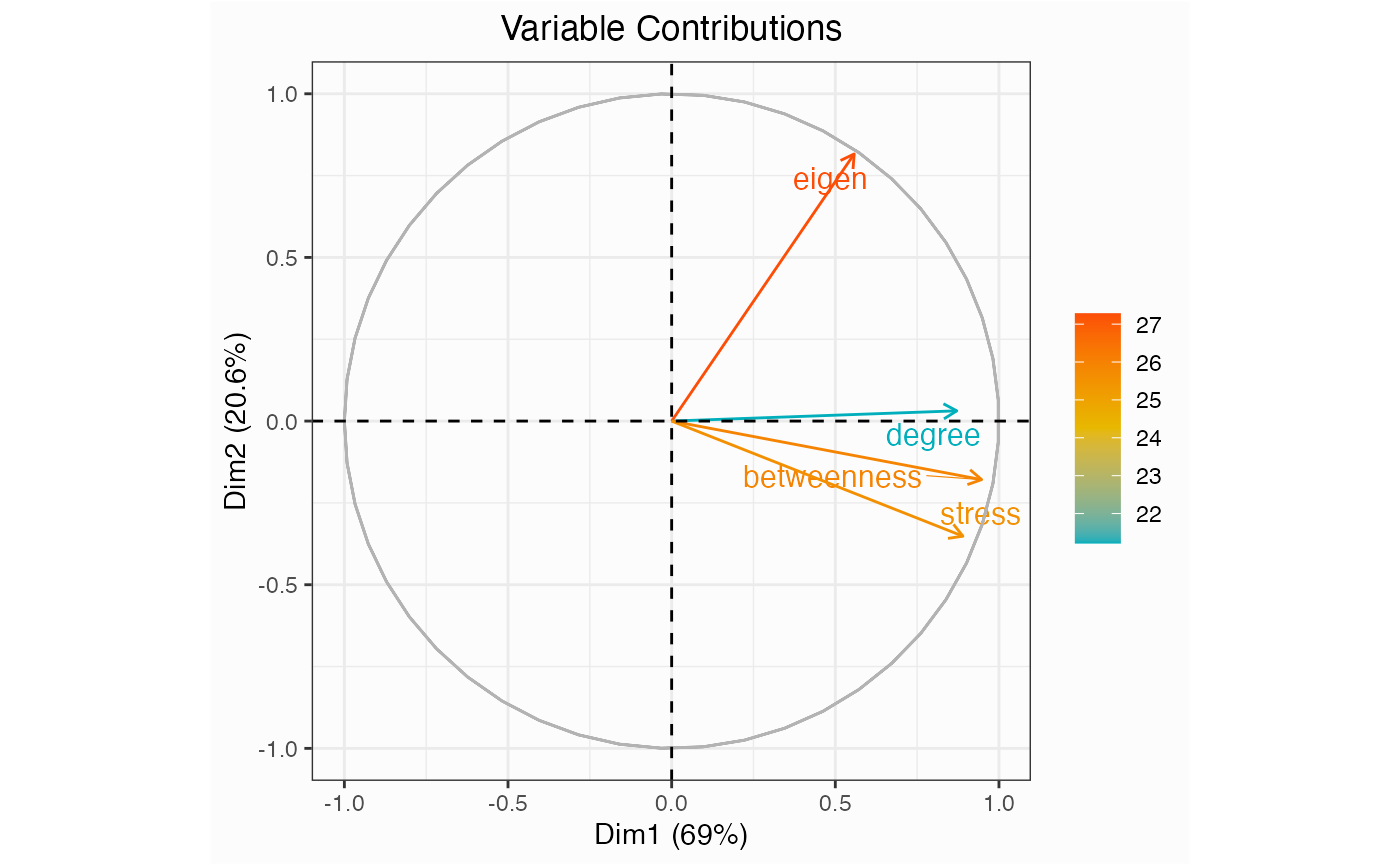

network.pca.contri(network)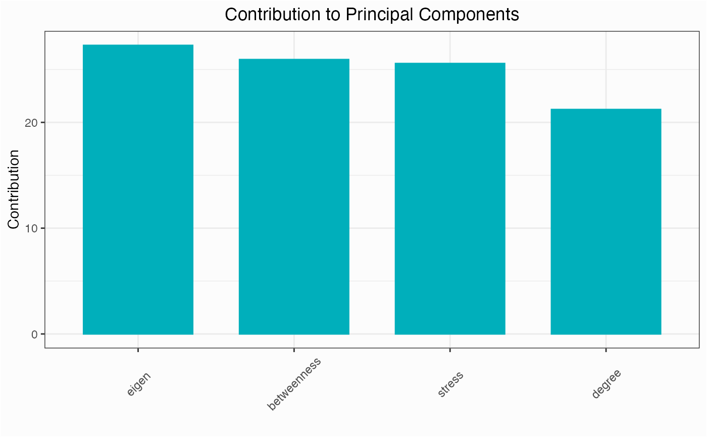

network.pca.varexp(network)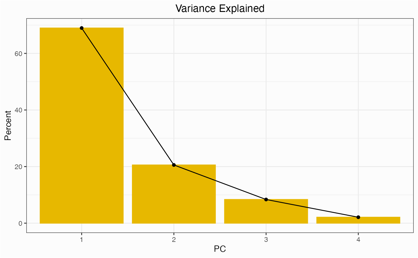

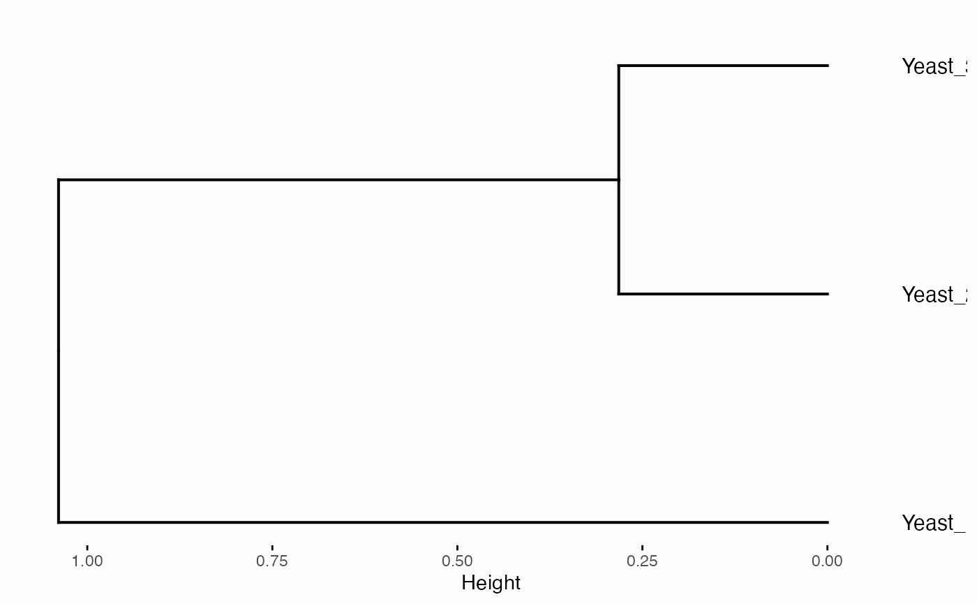
network.pca.hclust(network)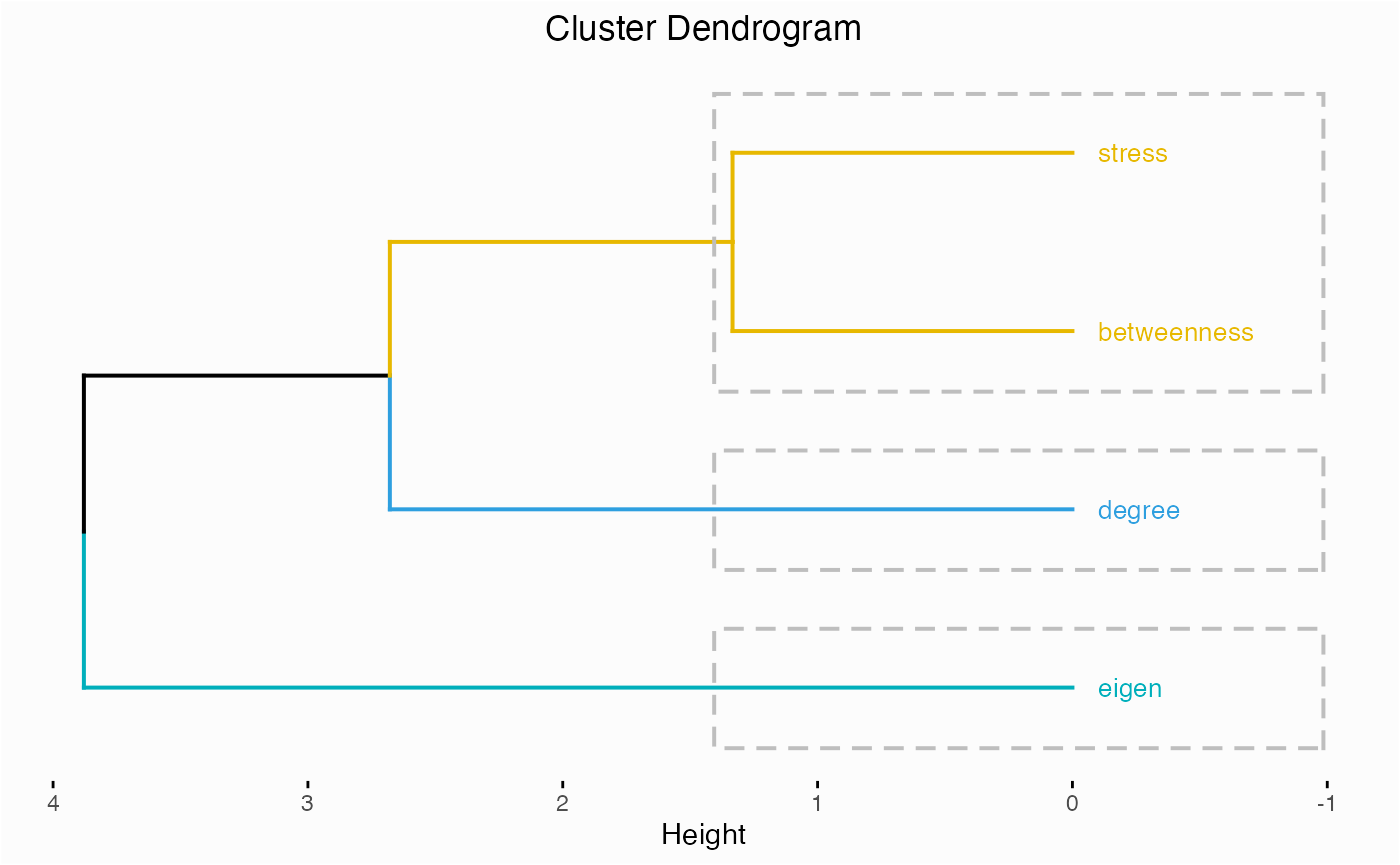

Centrality Distribution

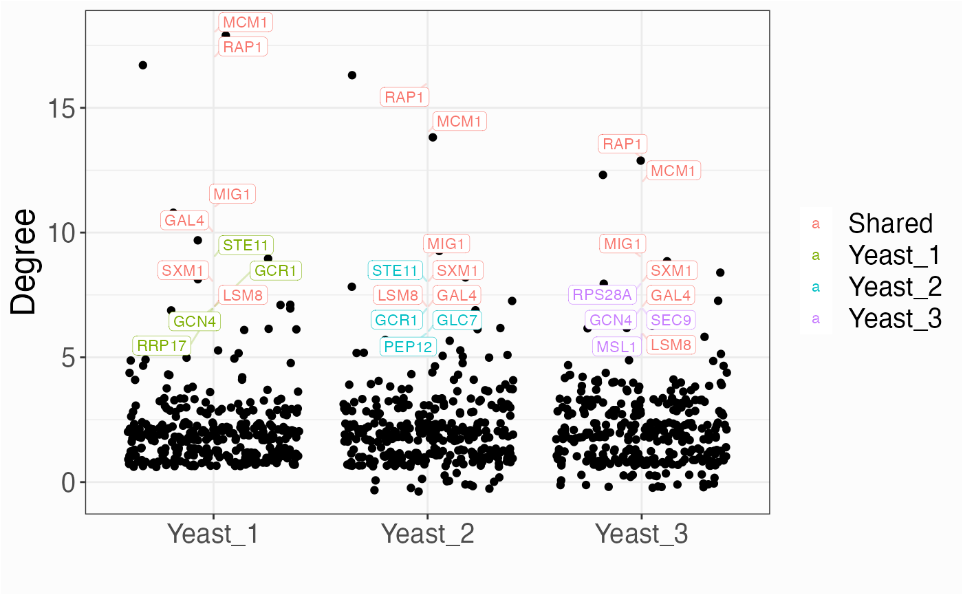
networks.cdistr(networks, metric="degree")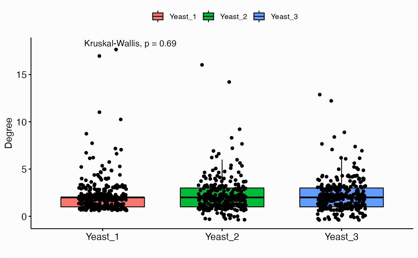

networks.cdistr(networks, metric="eigen", plot="density")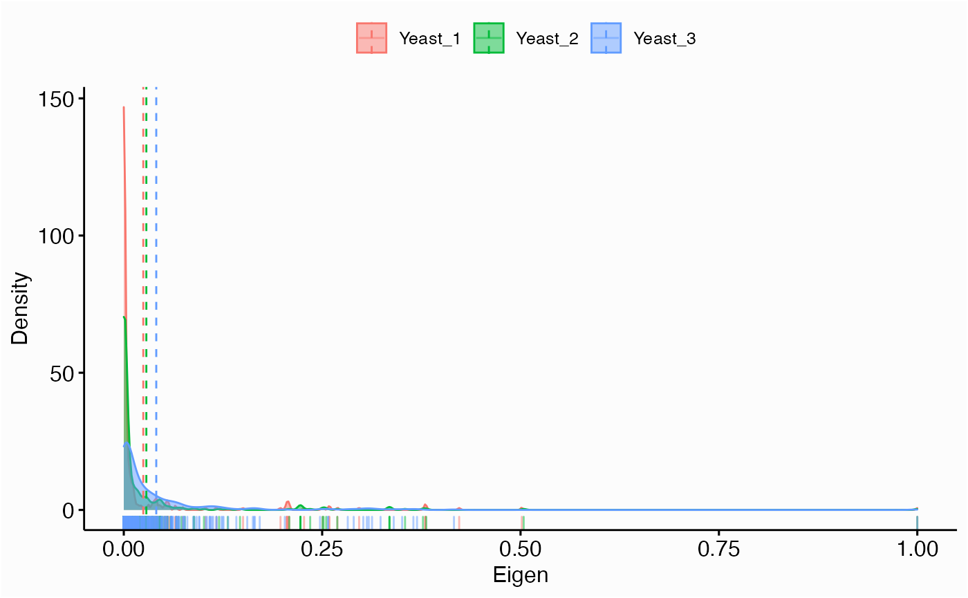

networks.cdistr(networks, metric="eigen", plot="ecdf")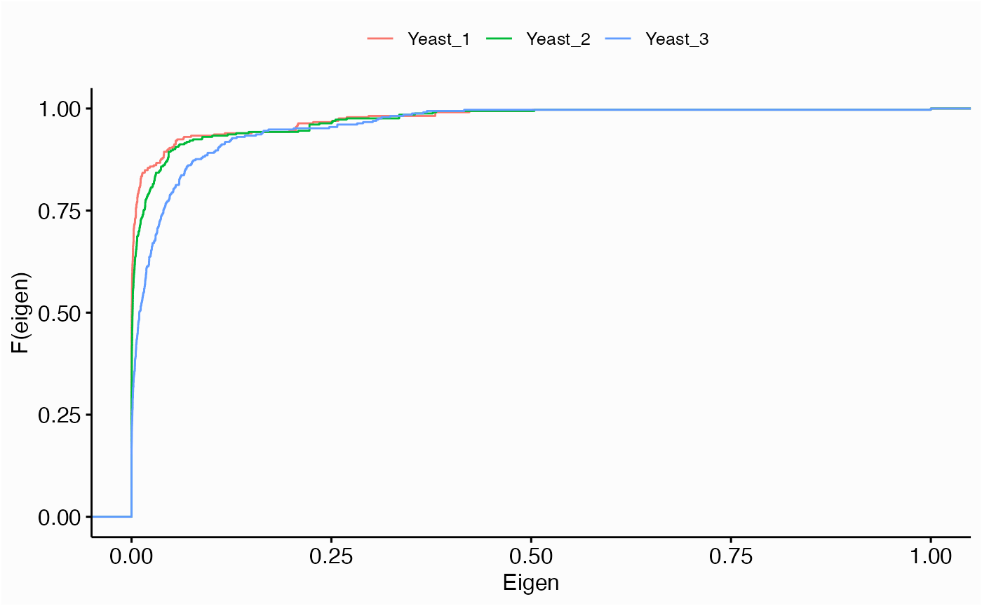

Hierarchical Clustering

networks.hclust(networks, metric="eigen", method="pearson")

Important Nodes

networks.tnodes(networks, metric="degree", top=10, symbols=TRUE, log=FALSE)

Centrality-based Enrichment

library(hypeR)
genesets <- enrichr_download(genesets="KEGG_2019", db="YeastEnrichr")
geneset <- genesets$`MAPK signaling pathway`
head(geneset)

[1] "RGA1"  "RGA2"  "STE50" "MSS11" "MID2"  "DIG1"

yeast.1 <- yeast.networks$Yeast_1

network.kstest(yeast.1, metric="eigen", geneset=geneset)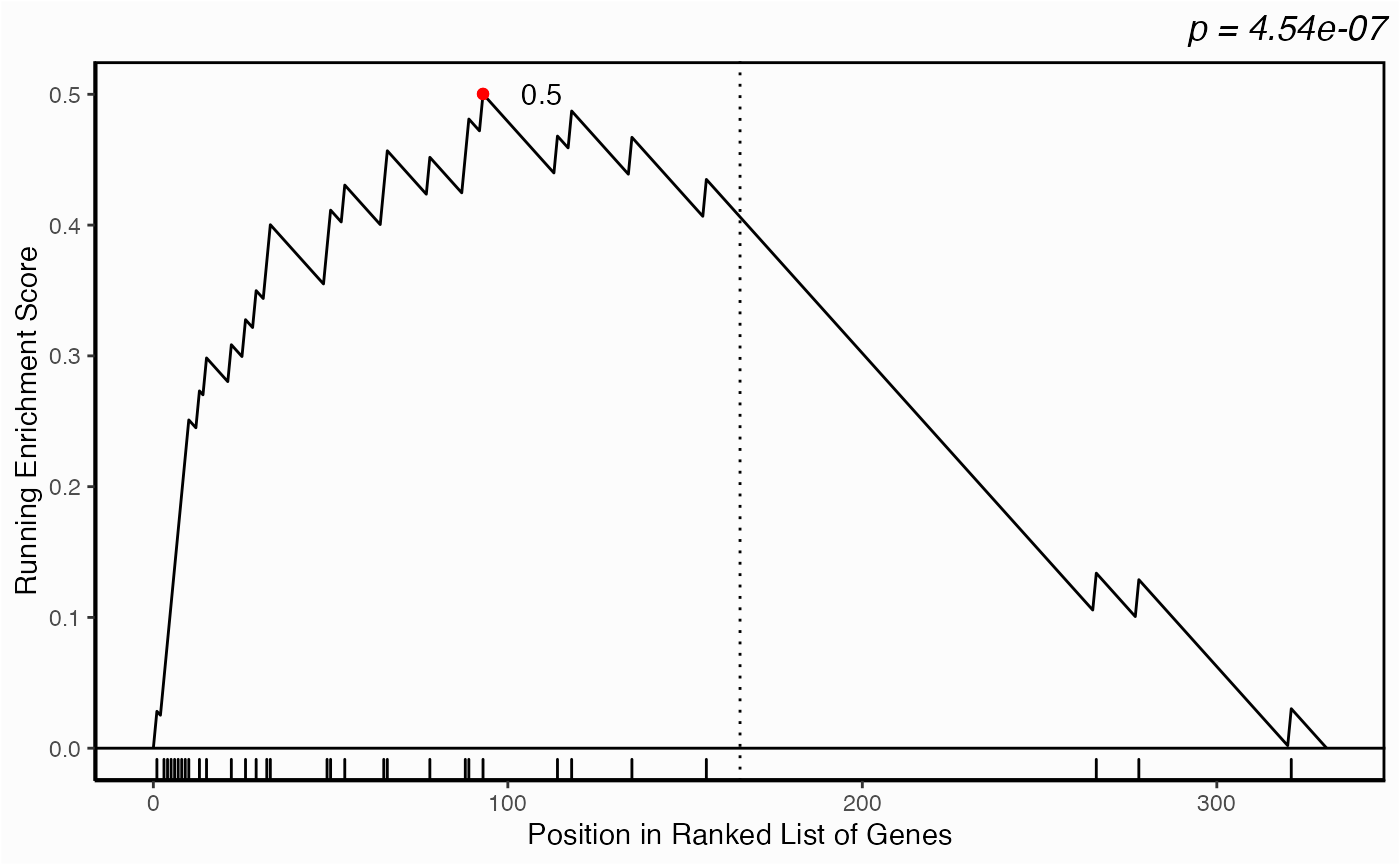

p <- lapply(yeast.networks, function(x) network.kstest(x, metric="eigen", geneset=geneset))
p <- mapply(function(px, label) {
   px+ggplot2::labs(subtitle=label)
}, p, names(yeast.networks), SIMPLIFY=FALSE)
ggpubr::ggarrange(plotlist=p, ncol=1, nrow=3)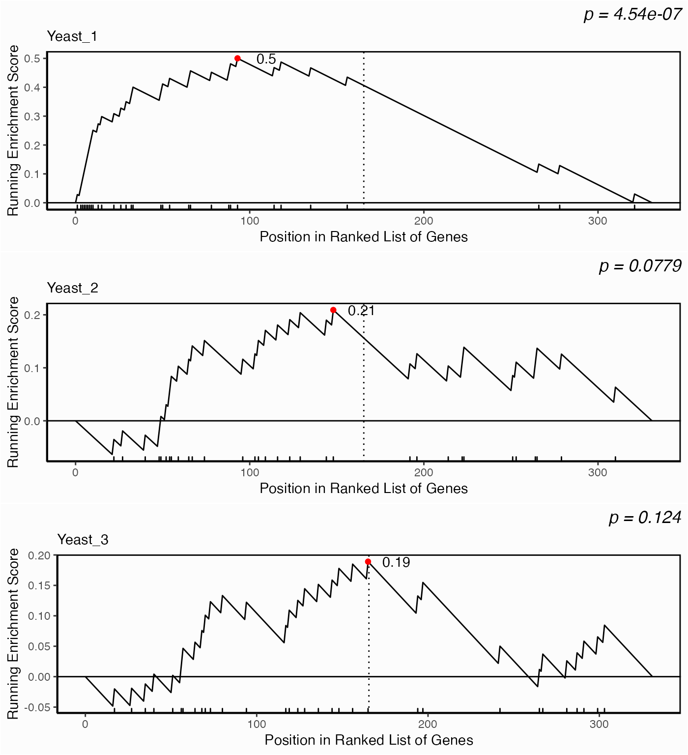

Comparing Centrality Ranks

ggwrs(100, p=5)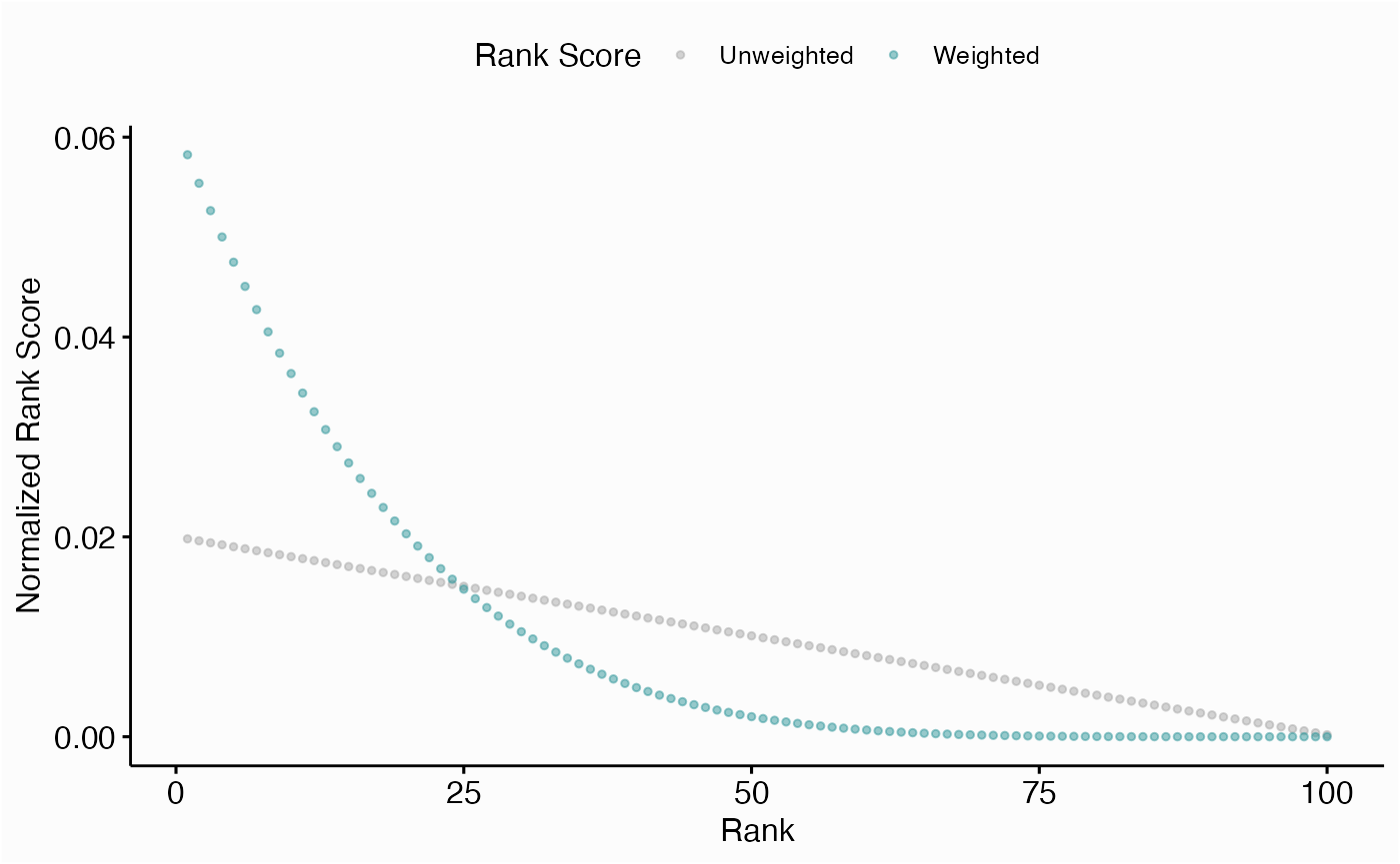

networks.diffc(yeast.networks, metric="eigen", top=25, p=5)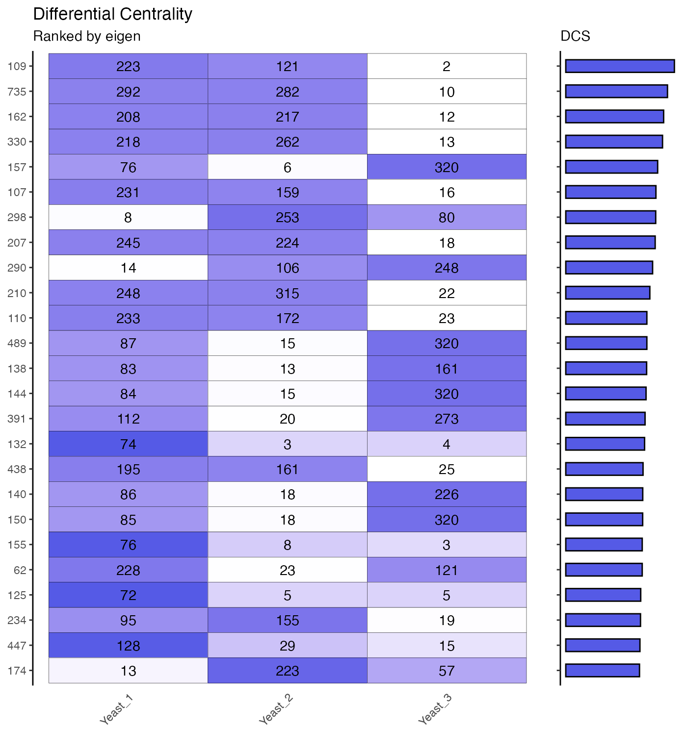

yeast.3 <- yeast.networks$Yeast_3
yeast.3$get.symbols("109")

[1] "LSM8"

yeast.3$plt.subnetwork(ids=c("109"),
                       degree=3,
                       use.symbols=TRUE,
                       node.size="eigen",
                       node.color=list("lfc_mrna", cfx(c("blue", "white", "red"))),
                       node.border=list("snp_frq", cfx(c("#e9e9e9", "black"))),
                       node.shape="is_tf")

Centrality Measures